Archive

Archive for the ‘what i’ve been doing’ Category

SMW11 Paper submitted

March 29th, 2011 2 comments

We have recently been working on a paper directed towards the Social Mobile Web 2011 workshop in Barcelona, Spain. A 4 page paper which is really a position paper, with some preliminary results:

Initial SMW2011 Submission

The main focus of the paper was to demonstrate that considering hierarchy in the mechanism for routing would improve the results compared to BubbleRAP, as the extra knowledge would give the algorithm an advantage. We called our algorithm BubbleH (details) and it used Hierarchical Greedy Clique Expansion (H-GCE) to discover communities.

BubbleH vs. the rest

March 15th, 2011 2 comments

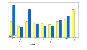
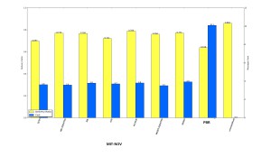
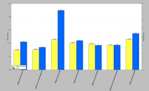
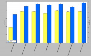
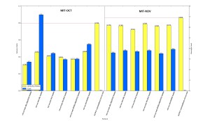
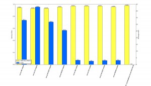
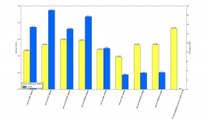
After a few iterations of bug fixes in the Bubble H code, it finally gave some sensible results. Shown below for MIT-OCT and MIT-NOV, where the community finding was done using a training set, and the test was done on the test set. Results are compared with the previous CFAs and also the  routing schemes we originally compared to (Bubble, PBR, Prophet, Unlimited Flood). GCEH was run multiple times with varying parameters, and the output chosen to drive BubbleH was chosen by picking a good looking result, this is a flaw in the process.

For MIT-OCT, the data in mit-oct-training.gce_output_K4_ST0.5_MAP0.5_e0.25_0.2.dat was used, which looks like:

  0(101)
  |
   - 1(71)
  |
   - 4(40)
  |  |
  |   - 2(16)
  |  |
  |   - 3(20)
  |  |
  |   - 5(28)
  |
   - 6(63)
  |  |
  |   - 7(47)
  |  |  |
  |  |   - 8(24)
  |
   - 9(66)

For MIT-NOV the data in mit-nov-training.gce_output_K3_ST0.5_MAP0.5_e0.15_0.2.dat was used, which looks like:

  0(101)
  |
   - 1(39)
  |  |
  |   - 2(16)
  |  |
  |   - 3(22)
  |  |  |
  |  |   - 4(14)
  |  |
  |   - 5(8)
  |
   - 6(30)
  |
   - 7(24)
  |
   - 8(63)
MIT-NOV

MIT-OCT

MIT-NOV

MIT-NOV

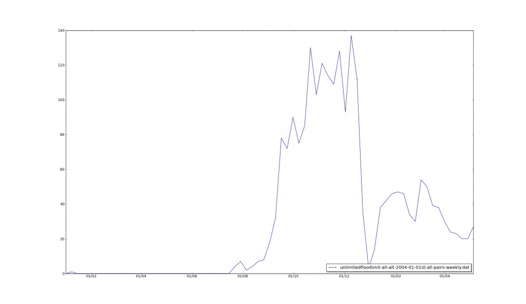
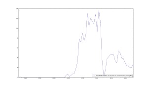
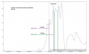
It is clear that MIT-NOV seems to have a better delivery ratio overall, this is probably due to the increased activity in December (MIT-NOV-TEST), compared to that in November (MIT-OCT-TEST), as seen in the activity plot below.

The average number of connections (bluetooth contacts) per week in the MIT Dataset

The average number of connections (bluetooth contacts) per week in the MIT Dataset

A thorough investigation would mean running the output of the many parameters used for the GCEH algorithm, and running the simulation over the whole lot – complicated, but possible.

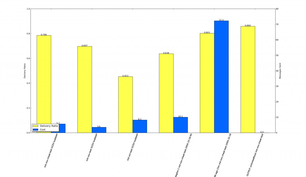
UPDATE: Using MIT-NOV-CHEAT dataset – i.e. allowing the use of data from the test period, gives a much better result – see below.

MIT-NOV-CHEAT

MIT-NOV-CHEAT

The candidate hierarchy was taken from similar parameters as previously: edge_list.dat.gce_output_K-3_ST-0.5_MAP-0.5_E-0.15_Z-0.2.dat which looked like:

  2(77)
  |
   - 0(52)
  |  |
  |   - 1(18)
  3(79)

This was slightly different from the previous hierarchies, in that it has less communities, but it demonstrated an accurate looking community structure – i.e. 3 communities. The results indicate that BubbleH does better here than previous attempts, which is encouraging. I also tried attempted to run the KCLIQUE version of BubbleRAP, but, as discussed before, it cannot find any communities in the training+test period.

Categories: experiments

BubbleH

March 10th, 2011 4 comments

It took a while to get the implemented version of BubbleH to run properly, it also took a while to get the GCEH algorithn (as supplied by Conrad) to work, however the core of BubbleH is as below:

public void onConnect(Process p, Simulation s) {
  // do the business
  List toSend = new LinkedList();
  BubbleHProcess process = (BubbleHProcess) p;

  // foreach message in my buffer
  for (BubbleHMessage message : my_buffer) {

    /**
     * Identify smallest community that Self and Destination share =
     * Bridging Community
     * */
    int bridge_community = BubbleHeirarchyOracle.bridgeCommunity(this
        .getNode().getID(), message.dest, my_properties);

    // if encountered node is destination
    if (p.getNode().getID() == message.dest) {
      // pass it on to them.
      toSend.add(message);
    } else {
      if (((BubbleHProcess) p).hasSmallerCommunity(message,
          bridge_community)) {
        // if P is in community with message.dest, that is smaller
        // than BC
        // pass message
        toSend.add(message);
      } else if (process.getCommunities().contains(bridge_community)) {
        if (process.getlocalRank(bridge_community) > getlocalRank(bridge_community)) {
          // if p.localrank for BC is higher than this.localrank
          // pass message
          toSend.add(message);
        }
      } else {
        // process is not destination, is not in a smaller community
        // with the destination, and is not in the bridge community,
        // therefore we do not pass the message to it
      }
    }
  }
  for (BubbleHMessage message : toSend) {
    my_transmittedCount++;
    message.hopCount++;
    s.sendMessage(this, process, message);
    my_buffer.remove(message); // not sure if this is strictly part of
    // BubbleRap, however to get anything like
    // the cost figures they quote, it seems
    // like the only way!
  }
}

In many cases, the bridging community will not be found, and therefore any node which at least has a community with the destination will get the message. However, one option is to make sure that every node is a part of one global community, this will have the effect to allowing the messages to start off in the right direction. But has the negative effect of adding more cost, as it really only does the same thing as the global rank does in Bubblerap.

Results below seem to reflect the poor heirarachy structure generated by GCEH.

BubbleH results for MIT-OCT-TEST along with the previous results, using training period MIT-OCT-TRAINING

BubbleH results for MIT-OCT-TEST along with the previous results, using training period MIT-OCT-TRAINING

bubbleh-mit-nov

BubbleH results for MIT-NOV-TEST along with the previous results, using training period MIT-NOV-TRAINING

Whilst the results seem poor, I believe that this is just an artefact of the GCEH output, the next step is to tweak the algorithm to give better heirarchical results. Also it might be sensible to test all of these algorithms on another dataset, to give some comparison for different types of networks (e.g. cabspotting?). Also, now that we have the social sensing dataset, it might be a good idea to see if it gives similar results.

The output of GCE for MIT-OCT-TRAINING is as follows – It is in the format:

community_id-parent_community: node ... list
# options
# {'phi': 0.25, 'threads': 5, 'max_times_spoken_for': 1, 'minCliqueSize': 3, 'num_realizations': 100,
'epsilon': 0.14999999999999999, 'perturb_alpha': 0.20000000000000001, 'minCliqueEdgeWeight': 0.0,
'similarity_threshold': 0.90000000000000002, 'outfile': None, 'min_appearance_prop': 0.5, 'intNodeIDs': False, 'file': None, 'alpha': 1.0}
74-0: 91 88 66 90 83 86 100 85 21 22 46 40 41 7 6 75 102 103 93 101 95 10 15 14 16 18 30 61
119-0: 2 30 16 46 47 6 61 43 41 91 88 63 8 102 83 75 101 95 94 67
160-0: 6 16 46 30 88 91 75 63 7 67 102 83 93 101 95 94 85
193-0: 61 88 90 83 86 100 85 47 43 41 5 6 8 102 103 93 101 95 97 78 91 10 15 14 16 18 30
263-0: 25 16 30 3 91 88 74 5 102 93 101 97 10
297-0: 16 30 3 41 91 88 63 67 102 2 100 101 74
335-0: 25 10 30 28 62 41 91 3 74 65 102 72
397-0: 38 17 61 46 31 30 102 91 80 101 93
433-0: 17 16 46 30 61 71 91
513-0: 24 30 59 58 23 46 54 45 29 60 61 89 64
612-0: 24 39 45 20 61 46 32 76 30 36 19 12 79 91 84
659-0: 24 45 61 46 30 42 36 19 12 70 91 87 84
726-0: 11 21 16 55 18 30 61 46 6 91 101 102 94
764-0: 12 61 46 56 45 36 77 98 30 91 100
806-0: 12 46 37 36 61 70 91 68
846-0: 27 46 55 30 37 61 6 102
910-0: 60 61 80 81 84 24 25 23 46 45 29 102 100 91 58 16 19 54 30 36 53 34 32
961-0: 91 20 58 23 46 54 30 51 36 29 60 19 79 32 61 81 84
1010-0: 91 23 38 19 46 54 30 51 53 60 61 79 102 80 81 87 84
1106-0: 89 68 87 84 24 20 46 45 42 4 77 76 70 79 39 12 98 19 32 56 37 36
1113-1106: 24 39 12 19 32 45 42 36 76 46 4 70 68 87 84

MIT-NOV-TRAINING  is below:

# options
# {'phi': 0.25, 'threads': 5, 'max_times_spoken_for': 1, 'minCliqueSize': 3, 'num_realizations': 100, 'epsilon':
 0.14999999999999999, 'perturb_alpha': 0.20000000000000001, 'minCliqueEdgeWeight': 0.0, 'similarity_threshold': 0.90000000000000002,
'outfile': None, 'min_appearance_prop': 0.5, 'intNodeIDs': False, 'file': None, 'alpha': 1.0}
72-0: 61 88 63 67 83 86 85 21 47 43 41 5 6 8 75 102 90 100 101 95 97 78 91 10 15 14 17 16 30 103
116-0: 61 88 63 83 80 25 21 46 47 41 7 6 8 75 91 90 93 101 102 97 78 10 14 17 16 18 31 30 53 34
165-0: 61 88 63 83 69 80 86 100 25 21 46 7 75 102 90 93 101 94 97 78 91 10 15 17 55 30 103
219-0: 61 63 69 21 46 47 41 6 91 102 90 100 101 94 97 78 11 10 13 15 55 30
284-0: 10 86 16 18 30 61 41 102 88 63 25 66 91 101 95 74 72
361-0: 11 25 91 10 46 30 62 41 61 3 65 102 101 72
402-0: 10 30 28 41 91 62 74 52 72 102 101
473-0: 38 16 46 30 41 61 80 92
507-0: 91 54 30 41 61 73 66 102
545-0: 39 12 46 30 42 91 82
587-0: 102 57 4 72
638-0: 61 88 67 47 41 2 5 7 74 91 90 100 102 78 10 15 14 16 18 31 30 51 103
716-0: 25 38 61 46 54 30 51 53 41 102 16 91 80 81 87 79
800-0: 50 60 61 89 68 87 84 24 92 20 48 23 46 45 42 4 77 76 70 101 79 39 12 59 58 98 19 32 56 37 36 53 54
853-800: 12 61 46 45 36 76 89 79 68 101 19 84 4
944-0: 60 61 80 81 84 24 25 23 46 47 45 29 91 101 102 58 16 19 54 30 36 53 34

So in the above, there is lots of communities which have no parents. So I forced the output to have one global parent which contains all communities:

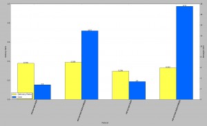
BubbleH with forced parent community, and without, using MIT-NOV and MIT-OCT test periods, based on relevant training period

BubbleH with forced parent community, and without, using MIT-NOV and MIT-OCT test periods, based on relevant training period

This shows a little improvement in delivery ratio, and increases the cost substantially.

Categories: what i've been doing

BubbleRAP using Heirarchical Community Structure

March 3rd, 2011 4 comments

The existing BubbleRAP mechanism works as follows:

on N connected with encountered node P
for each message M (for destination D) in buffer of N
if P == D
    pass message M to P
else
    if N and P share a community with D
        if LocalRank(P) > LocalRank(N)
            pass message M to P (and delete from buffer)
    else
        if (P shares a community with D) OR (GlobalRank(P) > GlobalRank(N))
            pass message M to P (and delete from buffer)
// keep message

The proposed version of Bubble-H (Bubble Heirarchical) works as follows

on N connected with encountered node P
for each message M (for destination D) in buffer of N
if P == D
    pass message
else
    if P is in a CLOSER community, that also contains D
        pass message M to P
    else if P and N share CLOSE community with D
            if(LocalRank(P) > LocalRank(N))
                pass message M to P
            else
                keep message
    // we need to still push messages to the top when there is no overlap
    else if(P is in a BRIDGING community with D, that N is not)
      pass message M to P
    else
      keep message

Bubble-H as above uses the notion of CLOSE(R) communities, and BRIDGING communities:

heirarchicalclustering-1

  • A CLOSER community, is the one that is lower down in the hierarchical structure of communities, for example, when N has the message destined for O, on meeting P, he would pass the message, as P is in a community lower in the hierarchy. Being CLOSER suggests that P is somehow more likely to be connected to O.
  • The shared CLOSE community is one that is low down in the heirarchy scale, that the destination is a member of, but that both nodes also share. They compare local ranks to decide who should have the message. For example. N and M share a CLOSE community with O and P.
  • A BRIDGING community, is at a lowest point that  bridges a gap between branches of the structure, in the example, the community C2 containing CDEA, GF and H, would be considered a bridge. (not the best example?). This is handy for when a node who is not in a low level community with the destination needs to get the message closer.

I think there might be something missing from this new algorithm, and I am not convinced it is any different to the existing BubbleRAP protocol, especially as nodes are not clustered hierarchically.

A note on hierarchical GCE: this algorithm produces communities that are hierarchically organised, however, the nodes within these communities can and will overlap, so that a node in a community in one partition of the tree, may also appear in a community on the other side, which means I have now realised that the illustration above is not a correct representation.

UPDATE (3/3/11): Pádraig’s comments make sense, and so the following is a better algorithm:

on N connected with encountered node P
for each message M (for destination D) in buffer of N
Identify bridging community (BC), smallest community containing N and D.
IF P ==D
   then pass the message
ELSE IF P shares a community with D that is smaller than BC
    then pass the message.
ELSE IF P is more central in BC than N
    then pass the message.

UPDATE (7/3/11): I have managed to get Conrad’s code to run today  and output the correct data, and it seems that the output is very different from what I had imagined; the MIT-Nov-Training dataset produces lots of non-heirarchical communities, and one or two parent-child structures (depending on parameters) – this means that in some/most cases, there will nodes who do not have bridging communities.

I am currently implementing BubbleH in the simulator and need to decide what to do in the case of no bridging community; two choices as I see it are: When a bridging community is not found either

  1. use global rank (as per original bubble rap), or
  2. Keep message until a bridging/smaller community is found.

My favourite is option 2, as this helps to hold the message by default, until a useful encounter comes along (a small world property?).

Vector clocks to drive delay tolerant networking

March 1st, 2011 3 comments

Vector Clocks can be used to build a knowledge of the network surrounding each node, from the local perspective of that node. This means that it would be possible to calculate some metrics about the global network, at each individual node. However, we already know [1] that in human networks, the 6 hour degree approximates the betweeness centrality of the node, which can be used as a useful metric for routing [2], so why should we complicate things further?

Benefits of vector clocks

Maintaining a vector clock [3] for each node encountered can give us extra information about the network. Assuming in our vector clock updates, we also transmit information about the network as seen by each node, we can tell both the structure of the network, and a number of extra things about the network that simply counting degree cannot.

Each node can know how out of date other nodes are, simply by checking it’s records, and seeing when an update was last received about that node, this gives some notion of distance from itself to other nodes (a.k.a. ball of radius, latency).

Indirect paths and essential links can be deduced at a global level by looking at the routes that are used to update vector clocks; where an update is received about an unknown node during an encounter, we can mark the encountered node as a possible carrier for the unknown node. And where one node is always used as a conduit for information updates about certain nodes, we know that it connects some other portion of the network.

The rate that other nodes update us with information (update rate) gives us a notion of how often contact is made with that node, the update amount, tells us how much knowledge about the network that node delivers . A node that has a high update rate is one that is encountered often, and one that has a high update amount may be well connected to other portions of the network.

Derived knowledge

Using these metrics, we can start to make other observations about the network. We now have sufficient information to attempt to predict future events [4][5]; Using the knowledge of update rate and out-of-dateness We may anticipate future encounters, based on the notion of periodicity [1], or perhaps even by simple Markov chains [6].

We can also try to calculate a notion of distance from one node to another using the update amount, out-of-dateness and out knowledge of the network structure. A nodes knowledge of the network also allows it to calculate things like it’s own centrality, degree and community membership, as well as giving it hints as to the same metrics for other nodes.

Vector clocks for location

Extending the idea further, it would be possible to share information about node movements along with network structure. Assuming nodes could detect their locations using some globally known scheme (e.g. simply using a grid-based approach to specifying location based on Latitude/Longitude), the vector clock updates can pass along updates about the last time a node visited a location, and perhaps the duration of the visit. This, combined with updates from other other nodes about their movements can give each node a picture of movements of other nodes. This in turn would allow us to make predictions[4][5] about where nodes will be in the future.

Usage

The combination of these metrics, gives us rich information to provide to a routing scheme, for example, it may be possible to adapt CAR [7] to use these metrics in it’s calculations, or a hybrid approach to BubbleRAP [2], where the global and/or local rank are based on these metrics. We may also want to devise our own scheme for routing based on this specific knowledge, however there are a large number of schemes already proposed, and it would seem  sensible to improve an existing scheme, rather than create yet another one.

Refs

1. Williamson G, Cellai D, Dobson S, Nixon P. Self-management of Routing on Human Proximity Networks Spyropoulos T, Hummel KA, eds. 2009;5918:1-12. Available at: http://www.springerlink.com/index/10.1007/978-3-642-10865-5 [Accessed July 7, 2010].

2. Hui P, Crowcroft J, Yoneki E. BUBBLE Rap: Social-based Forwarding in Delay Tolerant Networks. Networks. 2008:241-250. Available at: http://portal.acm.org/citation.cfm?doid=1374618.1374652.

3. Kossinets G, Kleinberg J, Watts D. The structure of information pathways in a social communication network. In: Proceeding of the 14th ACM SIGKDD international conference on Knowledge discovery and data mining – KDD ’08. New York, New York, USA: ACM Press; 2008:435. Available at: http://portal.acm.org/citation.cfm?doid=1401890.1401945.

4. Song C, Qu Z, Blumm N, Barabási A-L. Limits of predictability in human mobility. Science (New York, N.Y.). 2010;327(5968):1018-21. Available at: http://www.ncbi.nlm.nih.gov/pubmed/20167789.

5. Ashbrook D, Starner T. Using GPS to learn significant locations and predict movement across multiple users. Personal and Ubiquitous Computing. 2003;7(5):275-286. Available at: http://www.springerlink.com/openurl.asp?genre=article&id=doi:10.1007/s00779-003-0240-0 [Accessed July 31, 2010].

6. Musolesi M, Piraccini M, Fodor K, Corradi A, A. Supporting Energy-Efficient Uploading Strategies for Continuous Sensing Applications on Mobile Phones. Pervasive. 2010. Available at: http://www.springerlink.com/index/WH71427029706513.pdf [Accessed September 3, 2010].

7. Musolesi M, Mascolo C. CAR: Context-Aware Adaptive Routing for Delay-Tolerant Mobile Networks. IEEE Transactions on Mobile Computing. 2009;8(2):246-260. Available at: http://ieeexplore.ieee.org/lpdocs/epic03/wrapper.htm?arnumber=4585387.

Routing using communities

February 21st, 2011 2 comments

It is important to make sure that each community finding algorithm (CFA) gets a chance to compete on a level playing field, so that they can be equally tested.

The dataset is MIT Reality Mining, which starts in August 200? and ends in May 200?.

The Bubble RAP algorithm uses k-KLIQUE for community finding. The graph contains the core nodes in the dataset, edges are created when a contact is made between two nodes, and labelled with the total time connected between the two nodes. Edges are removed when the total time connected is less than a defined threshold. Then it detects the communities using a k-CLIQUE algorithm, where k = 3. The threshold used by Graham is 2 days. It is 4.5 days in the BubbleRAP paper.

MIT-OCT has been used extensively by Graham, along with MIT-NOV to test his algorithms, so we will continue to use that time period for testing. However, we must make sure that there is sufficient time for all clustering algorithms to make a good effort at finding communities. I believe this was down to the fact that there was activity recorded a large number of users in the dataset for these  time periods.

The figure below shows the average number of connections per week for the whole dataset.

The average number of connections (bluetooth contacts) per week in the MIT Dataset

The average number of connections (bluetooth contacts) per week in the MIT Dataset

A note about the MIT-OCT dataset: There are two groups of nodes in the dataset, those belonging to the CORE set, and the rest, which belong to the encompasing ALL set. A node is determined to be in the CORE set if it is part of the MIT Reality Mining study, and is reporting readings. A node that is not in the CORE set, but is in the ALL set, represents a device that has been spotted by a node in the CORE set, but that is not known about apart from it’s contact trace. These are normally considered separate to the routing process, as it would not be possible to communicate with that node.

So, for the first experiment, each algorithm will generate communities from 01 Aug 2004 until 27 Sep 2004, and 01 Aug 2004 until 18 Nov 2004. The test period will be  27 Sep 2004 to 25 Oct 2004 and 18 Nov 2004 to 15 Nov 2004.

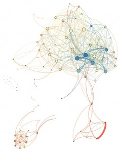
The image below shows the network generated in the MIT October training period. Some of the low weight (connected time) edges are removed for clarity. It appears to have three groups of nodes.

Visualisation of MIT OCT Training edge list. Edges are weighted by the amount of time nodes are connected, with low weight edges removed for clarity. Nodes are sized and coloured by degree.

Visualisation of MIT OCT Training edge list. Edges are weighted by the amount of time nodes are connected, with low weight edges removed for clarity. Nodes are sized and coloured by degree.

Some options for community finding algorithms:

  • Should the graph they all work on be limited by the threshold period?
    • Justification for this is that BubbleRAP determines this to be important
  • Whether or not to use CORE|ALL nodes
  • If the CFAs cannot successfully find communities for the training period, we will need to experiment with time periods that suit all algorithms.

The table below shows the results of community finding on the training datsets mit-oct and mit-nov, apart from KCLIQUE which performs very poorly before the end of December for any threshold value, so for the test period,  01 Aug 2004 to 31 Dec 2004 was used to calculate the communities.

Dataset # Communities Average Size
MIT-OCT-TRAINING – 01 Aug 2004 to 27 Sep 2004
KCLIQUE t=2days – to 31 Dec 2004 8 7
MOSES 7 35
MOSES adjusted graph * 1 12
GCE 4 60
ABL adjusted graph * 11 3
ABL 113 7
MIT-NOV-TRAINING – 01 Aug 2004 to 18 November 2004
KCLIQUE t=2days – to 31 Dec 2004 8 7
MOSES 8 42
MOSES adjusted graph * 3 7
GCE 2 51
ABL adjusted graph * 41 3
ABL 99 8

* adjusted graph means that some edges were removed from the edge list before passing to the algorithm, in this case, edges where the total connected time of nodes was less than 1 day.

Bubble results for test period Oct and Nov 2004, with training periods 01 Aug 2004 to 27 Sep 2004, and 18 Oct 2004 respectively.

Bubble results for test period Oct and Nov 2004, with training periods 01 Aug 2004 to 27 Sep 2004, and 18 Oct 2004 respectively.

Bubble results for test period Oct and Nov 2004, with training periods 01 Aug 2004 to 27 Sep 2004, and 18 Oct 2004 respectively.

Bubble results for test period Oct and Nov 2004, with training periods 01 Aug 2004 to 27 Sep 2004, and 18 Oct 2004 respectively.

average-weekly-connections-alt

Average weekly connections, showing training period and test period for MIT-OCT and MIT-NOV

BubbleRAP routing using different clustering techniques

February 15th, 2011 6 comments

After a lot of wrangling with code, and spending a good deal of time reading through notes, etc. I was able to work out how to generate community clusters using LocationSim, and how to feed in clusters determined by other mechanisms.

BubbleRAP uses and adapted form of KCLIQUE clustering to generate community structures, along with a score of Betweenness centrality (referred to as Hui Ranking) globally and within clusters to drive the routing process. The adaption relates to the use of a contact threshold, (the Bubblerap paper uses 4.5 days, Graham uses 2 days), which specifies how long on average nodes must be in contact for them to be counted.

I adapted the clustering phase to use MOSES, GCE (using Conrad’s code) and the algorithm by Yong-Yeol Ahn, James P. Bagrow, Sune Lehmann in Link communities in complex networks which I have name ABL. At this stage I have tested only the basic algorithms against MIT-OCT and MIT-ALL node lists.

Dataset # Communities Average Size
MIT-OCT
KCLIQUE t=4.5days
KCLIQUE t=2days
MOSES 8 29
GCE 3 41
ABL 64 8
MIT-ALL
KCLIQUE t=4.5 days 6 6
KCLIQUE t=2 days 7 9
MOSES
GCE 1 101
ABL 16 19

I found that KCLIQUE does not find any communities for the small time slice in MIT-OCT, this could be because the threshold means that in the course of a month, participants do not spend alot of time together on average.  I will need to explore this further to verify this this.

MOSES and GCE perform badly on the denser, MIT-ALL dataset, and after speaking to Aaron and Conrad, it seems this can be expected with such a closely connected dataset. My next step is to try to use GCE using edge weights, to see if that makes a difference.

in order to get some idea of results for MIT-ALL MOSES and GCE, and MIT-OCT KCLIQUE, I used the communities from their opposite positions to populate the datasets, this meant I was able to simulate BubbleRAP for all cluster types for both MIT-OCT and MIT-ALL.

Another intersting thing I discovered, was Grahams implementation of  Bubble-Degree, which instead of using the Hui Ranking for communities, nodes are ranked by degree over a 6 hour time period. Bubble-Connections worked in the same way but the ranking is based on the number of connections in a 6 hour period. (Graham explains this in section 6.1.2 in his thesis, and in the comments of his code).

The results are below for all cluster types, and both datasets, using bubble-degree, and bubblerap. Also included is unlimited flood to show the maximum possible delivery between all pairs of nodes.

Results for Bubble and Bubble-Degree for dataset MIT-ALL, using KCLIQUE, MOSES, GCE and ABL

Results for Bubble and Bubble-Degree for dataset MIT-ALL, using KCLIQUE, MOSES, GCE and ABL

Results for Bubble and Bubble-Degree for dataset MIT-OCT, using KCLIQUE, MOSES, GCE and ABL

Results for Bubble and Bubble-Degree for dataset MIT-OCT, using KCLIQUE, MOSES, GCE and ABL

This seems to suggest that the clustering algoritm does have some effect on the routing algorithm, and further analysis may be able to show whether this is due to simply the difference in number/size of communities.

Other tasks to do:

  • Investigate recent improvements of Bubble Rap (if any)
  • Consider different network data  (e.g. can we run a similar analysis over a phonecall network?)
  • Tweaks to clustering algorithms?
  • Chase up SocialSensing dataset
  • Continue to think about Location Based Routing – is it feasable still?

Routing to the centre

February 2nd, 2011 2 comments

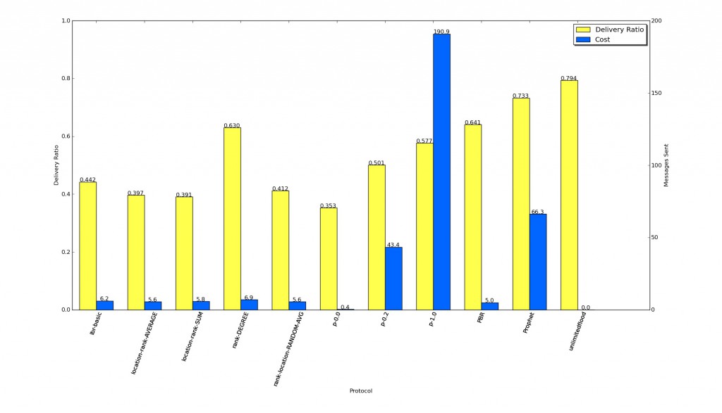
Further to the previous post, I have run some more simulations which include degree rank routing, where individuals are ranked in order based on their degree. I also updated LBR to allow for randomising rank scores, and ran this 25 times to get an idea about the ability for random ranking to deliver messages.

All routing methods shown for comparison.

All routing methods shown for comparison.

Interestingly,  routing based on degree only, gives a good delivery ratio. The average of the RANDOM runs performs slightly better than the more sophisticated LBR schemes, but not quite as good as LBR basic (which is the original ranking based solely on cell towers). This suggests to me that the mechanisms we are using to rank locations are not working, perhaps due to lack of rich enough data. It will be interesting to see how this dataset compares to other datasets.

Some new ideas

February 1st, 2011 2 comments

Met with Pádraig,  results so far are not complete, so we still need to:

  • Run routing based on ranked centrality only (i.e. the aggregate graph of all connections): Graham might have done this already. To give us a more complete picture of what routing towards the centre really looks like.
  • Do more randomised ranking runs, to see of random can come up with better routing rank than LBR.
  • Implement and test new LBR idea.

Next Step for LBR

Pádraig suggested a simple advancement for LBR:

Person A, has a  message for Person C, and has encountered Person B. A has to work out whether to pass the message on or not. Each node has  a probability matrix of visiting all locations at any time.

Probability matrix of nodes being at any given location

A makes his decision by calculating the dot product of his own locations against C’s locations, and comparing that to B’s calculation in relation to C. If the sum for the B.C is greater than A.C then A passes the message to B. The rationale being that when one encounters someone else, who is more likely to visit the same location as the destination person, then the message should be passed on, because they are more likely to see the other person.

There are some caveats….. TODO: buffer zone, future prediction, past history, recent(ness?), limited locations,

Some specific details/ideas/extensions to consider:

  • We need to consider how these probability matrices will evolve over time. A nodes probability matrix will change when he/it visits new places, or alters existing mobility patterns. Initially, we can use the computed data, but more refined versions should exhibit a real-world scenario of unpredictable behaviour.
  • Determine a good threshold to use, so that messages are not sent between people of very similar rank/score, the rationale being that there may not be a benefit in passing it on, and therefore try to reduce overhead.
  • Limit the number of locations considered, to only those that are popular, this might boost the use of popular locations, in an attempt achieve a higher probability of a message being passed on.
  • Consider a more sophisticated mechanism to predict co-location with the destination node, or a better conduit/carrier node, by predicting future interactions with nodes based on past history.
  • It may also be important to show the possibility of real-world application, by implementing  a scheme for automatic dissemination and update of the probability matrix using the network itself. (related to  previous ideas about piggybacking meta-data using network/vector clocks, which themselves can be used as a source of routing metrics. e.g. recentness of contact, latency, update routes/speeds/times etc.)

Pádraig and I discussed the problems we may encounter in regards to peer review and justification of the work; in that the problem area is not well defined, and therefore we might have problems showing why this work is novel, and proving what our contributions are. To that end we need to explore the literature a little more, so we might be able to show a solid justification for the work, or alternatively, change our approach so it fits in better with other, better defined problems.

What sorts of messags are ‘delay tolerant’? Pádraig’s suggestion is that twitter messages, and facebook update messages might be delay tolerant, as a person may not need to receive all messages, and generally only want to get the latest updates, it does not matter if a few are lost along the way.

How do we define the urgency of messages, and the efficiency of the network? Perhaps one type of message can be delivered within 10 time periods, and still be considered to be relevant and within acceptable delivery time, but another message may need to be delivered within 1 time period, to ensure quality of service.

There is a categorisation issue too; where some messages can be considered one-to-one (direct messaging), some one-to-many (twitter update), many to many (local information) and many-to-one (sensor networks). We need to decide which of these we will consider. On this note, I said I would speak to Neil Cowzer, who is working on implicit group messaging, to see what his motivation is, and to see if he has a well defined problem space that he is tackling.

Another alternative that Pádraig suggested, was looking at social science approach, where we look at the heuristic approaches to routing in complex social networks. Pádraig’s suggestion was that on some networks, we might be able to apply certain routing techniques, which do not work on others. The contribution would be defining, categrorising and testing new and existing combinations of network types and routing mechanisms. This would be an interesting route to take, but would mean a step back in my research, as I would need to do reading into this area. This would link up well with the work of Stanley Milgram, Granovetter and Watts & Strogatz etc. So I should re-read some of this work, but more importantly, take a look at the biggest cited, citing documents, to see where research might be heading now.

MIT Cell Tower Community Finding

January 19th, 2011 3 comments

Had a meeting with Pádraig; we discussed using MOSES to get the list of communities of cell towers.

To recap, two cell towers are linked, if during a contact (Bluetooth) between two people, they are spotted by either person. This generates a huge furball of when visualised. I installed MOSES on a server, and ran it on the graph generated from MIT Oct 2004. It produced 66 Communities. There are 468 nodes in the dataset. The average number of communities per node is 2.17.

Padraig suggested visualising the data, and colouring each community in turn, so that we might be able to get an idea about which communities we can remove (as they are too big), and will leave us with smaller subsets of the graph, which identify locations better.

We can then use these communities as the ‘locations’ in location based routing. We need to determine whether it matters if a node report multiple ‘locations’ at the same time.

I started to view the communities colours as suggested, but it still showed a very large furball, so I decided to see what happenned when the highly connected nodes are removed. In the image below, we can see that when the top  100 highly connected nodes are removed, it becomed clear that there are distinct groups of cell towers.
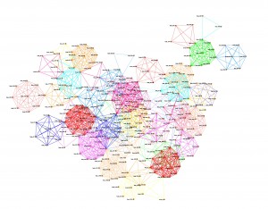
MIT Oct 2004, when two users see each other, the cell towers they see are linked. This version has the top 100 highest connected (degree) nodes removed.

MIT Oct 2004, when two users see each other, the cell towers they see are linked. This version has the top 100 highest connected (degree) nodes removed. Edges show community membership as given by MOSES.

I sent on the moses output, and list edges to Aaron McDaid and Daniel Archambault, who genereated the Euler diagram  below using Tulip.

the layout in the visualization is based solely on the communities found by moses. Tulip attempts to lay out the sets in an Euler diagram such that communities are placed nearby if they share nodes in common.
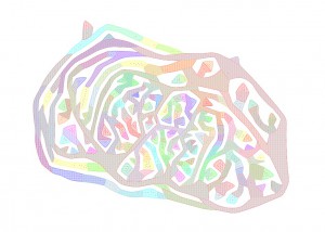
Euler Diagram generated using Tulip from the output of MOSES for cell towers connected in MIT Oct 2004.

Euler Diagram generated using Tulip from the output of MOSES for cell towers connected in MIT Oct 2004.

I have yet to speak to Aaron in more detail about what this diagram means, but if I have interpreted the visualization correctly, the similar coloured areas are collections of nearby nodes; seperated into distinct clusters, rather than overlapping ones. If it is possible to extract this clustering, it might provide exactly the location clustering we need, if we remove the very large clusters (light brown/green).

I took some time to review the way that cell towers are linked, to make sure that it was making a fair linking, ready for when MOSES did it’s thing. As it is, it is a little loose in how it determined whether two cells are linked, as it links all cells that are seen in an entire contact period. This means that cells that are linked when two people are travelling together. I plan to work on a more strict approach, where the duration of the cell sightings for each person are compared, and cells linked only when it is clear that they are at the same time. However, I continued using the results we already have.

The images below show the graphs, when the top N communities are removed. The size of the node relates to the number of times a cell tower is reported, using binning.

The most number of times a node is spotted is 9291, the smallest is 1, so
9291 - 1 / 10 bins = bin size of 929.
For example, if a node is spotted 1043 times, then it will be placed into bin 2.

The width of the edge relates to the number of times an edge is reported between its two vertices, again using binning. The most number of times an edge is spotted is 3676, minimum 1. The average however, is only 8.38, and the median is only 3, so the binning really only distinguishes the very highly seen nodes.

The colour of the edges is related to the community membership. Because nodes can be members of multiple communities, and therefore have multiple edges, I made the decision to create only one edge, and distinguish it using the concatenation of the community names (e.g. Community_0Community4…), so nodes that edges that make up the same communities, will have the same colour. This might not have been the best way to do it, but the software used does not show multiple edges between the same nodes. An alternative would be to make the width of the edge equal to the number of communities it represents.
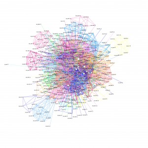
Minus 1 Community
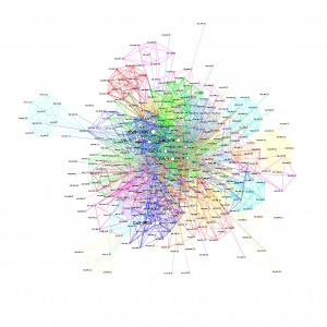
Minus 1 Community

Minus 15 Communities
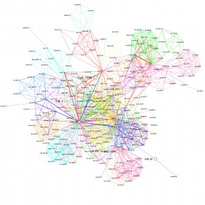
Minus 15 Communities

Minus 30 Communities
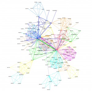
Minus 30 Communities

Minus 40 Communities

Minus 40 Communities

As communities are removed, the graph becomes clearer, where 40 communities are removed, it becomes more obvious that there are distinct communities and the high degree nodes are more obvious.

eps and png files for other numbers removed

The goal is; given any cell tower id, we can identify which community it belongs to, and by extension, the ‘location’ the node is at.

An idea I have for finally making this data usable, so that we have distinct communities. Ignore the top N communities (e.g. 30). Order each community by summed weight of edges, then take the highest degree node, and assign it to the community it belongs to, that has the highest rank, then remove that node from further consideration. Continue until all nodes are assigned to a community. This may need some more thought.