Archive

Archive for the ‘what i’ve been doing’ Category

MIT Contacts – Cell Tower stats

December 17th, 2010 2 comments

I processed the contact logs, rather than just the hop logs, and after ~6 hours it completed! Now all contacts in the whole MIT dataset have associated cell towers. If a cell tower could not be found for the contact duration, then a second search was done for a record of a cell tower finishing  in the previous hour. The timestamps are preserved so that they can be excluded later. The following shows the stats for this data, in regards to cell towers.

Row Count:	114046

Both Have Cells:		28804	 (25%)
Neither have cells:		34587	 (30%)
One side has cells:		50655	 (44%)
	From has cells:		30557	 (27%)
	To has cells:		20098	 (18%)
Nodes share cell:		4045	 (4%)
First start time:		Thu, 01 Jan 2004 04:03:17 +0000
Last end time:			Thu, 05 May 2005 03:39:29 +0100

This means that out of 114046 contacts between 01 Jan 2004 and 05 May 2005, only 4045 nodes report at least one cell in common at time of contact, but 28804 report different cells, and a further 50655 report cells for at least one of the nodes. This means, that if we assume that a one sided cell sighting at time of contact determines a cell sighting for both nodes, then we have cell towers for ~73% of  contacts.

The assumption is that if any of the cell towers seen in the contact period, then the nodes are considered to share a cell. However, this can be further refined if needs be, to be more strict, where a contact period is very long.

UPDATE:
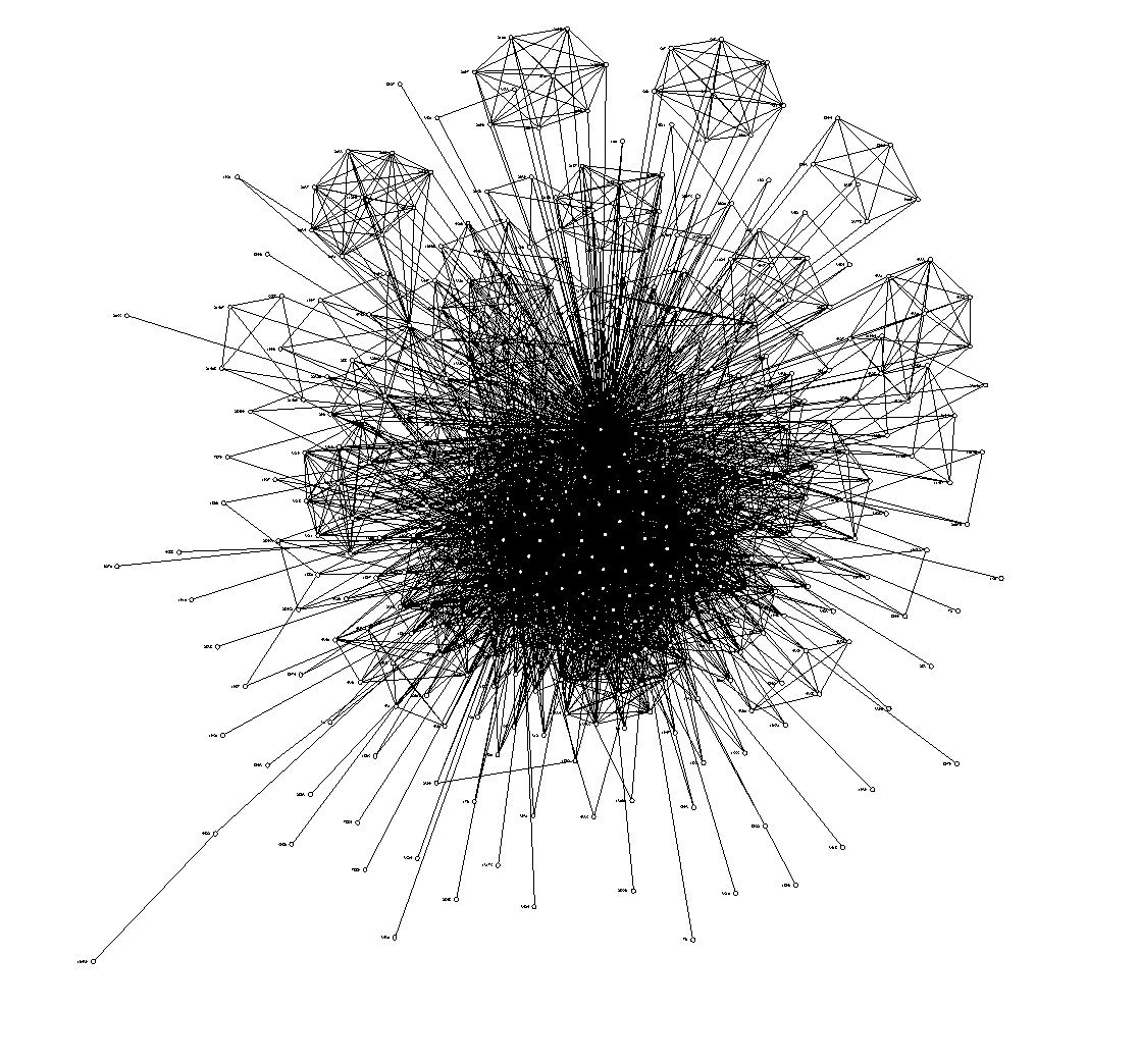
Below is a visualisation of the connected cell towers for MIT-Oct 2004, it it very confused and has a huge central mass, but there are clear connections of towers on the periphery. I think this can be further refined to be more strict about cell tower connections (as at the moment, the dataset contains more than 1 cell tower for any given contact period). Also, at the moment it links two cells even when two nodes are on contact for a long period of time, in which they could conceivably be moving together.
hairball-mit-oct-2004-cells

Cell towers where an edge is made when either node in a contact event has seen one of the cell towers.

Updated plots for Community Structure

December 14th, 2010 2 comments

In the last meeting I had with Pádraig we went through the spectral clustering technique, and discovered that there were some errors in my calculations of the the clusters. I took the time to re-do the community calculations,  and to run the tests again, to make sure all is correct. I used the MIT  dataset, and constrained it to the month of October 2004 (as before). Messages are created and initially sent at the first time step. The selected communities for each week are taken as the biggest group, which in practice were roughly the same set of connected nodes. I chose to omit the nodes with a value of 0.0 in the matrix (V) (see  data pipelines).

Delivery Ratio over time

mit-oct-start-community-lbr-lineplot

This plot shows the delivery ratio over time for MIT-OCT dataset, for LBR communities (where the community is taken from weeks 1, 2, 3, 4 and all 4 weeks), PBR, Prophet, Unlimited Flood and Random(1.0, 0.2, 0.0).

Final Delivery Ratio and Cost

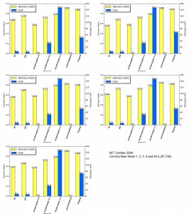
mit-oct-start-community-lbr-barchart

This chart shows delivery ratio and cost for each Protocol, note that unlimited flood does not report cost.


In these updated plots, it is encouraging to see that with the corrected community structure, LBR actually performs well, and in fact for the community structure in week 1, it performs better overall than PBR, with weeks 2, 3, 4, all, close behind. It is also good to see that LBR is beating Random 0.0, and 0.2 consistently. LBR week 1 Community also tracks a small way behind Flooding for a short while around 05/10 – 08/10 which is quite interesting. The communities are listed below (or can be viewed here), for further analysis.

UPDATE:

Having given this a little more thought, this is a little mis-leading, so I have generated new plots where all Protocols are constrained to the same community nodes. Unfortunately, this yields a similar spread of results between the protocols, as did the results that did not consider community structure. Only the structure discovered in week 1 increases the delivery ratio.

Delivery Ratio for each community, for each protocol

mit-oct-communities

This plot shows delivery ratios for each community generated from different weeks and all weeks in Oct 2004 for the MIT Reality Mining dataset

cost-dratio

This shows the final delivery ratios and costs for each protocol, for MIT OCT 2004, communitites

What I plan to do now is to go back to the ranking algorithm, and use the linked cells mechanism to re-calculate the rankings. It might also be useful to start thinking about being able to use the real-time location information (in this case cell towers/linked cell towers) in a routing algorithm directly. This would let us start to implement some simplistic location predictions.

I also created a clearer graph visualisation for the cell tower links, this shows that there is a componant that  encompasses a large percentage of the reported cells overall. If we were to consider this one location, it is possible that it covers a very large area.

connected-cell-towers_new

This shows the cell towers that are connected when at least 100 messages are passed and reported at both cell towers, edges are numbered where this is more than 300.

Cell tower connections based on contact events

December 10th, 2010 2 comments

Using the log of hop events, I was able to generate a list of cell towers being used at the time of the hop, from this I built a list of the cell towers that are linked in this way, with a count of the number of times they had been connected (linked_cell list txt, or linked_cells json version ). From this a created a graph where the weight of the edges is the count.

connected-cell-towersEdges with a weight (or number of times nodes passed a message and reported different cell towers) less than 100 are removed for clarity, the colour of the edges shows the weight of the edge increasing from blue to green.

The tool that I have used to visualise these graphs is called the network workbench, and it reports the following about the graph:

Nodes: 84
Isolated nodes: 9
Node attributes present: label
Edges: 149

No self loops were discovered.
No parallel edges were discovered.
Edge attributes:
Did not detect any nonnumeric attributes
Numeric attributes:
min    max    mean
weight     1    2700    103.42953

This network seems to be valued.

Average total degree: 3.547619047619045
Average in degree: 1.7738095238095228
Average out degree: 1.7738095238095228
This graph is not weakly connected.
There are 14 weakly connected components. (9 isolates)
The largest connected component consists of 67 nodes.
This graph is not strongly connected.
There are 61 strongly connected components.
The largest strongly connected component consists of 24 nodes.

Density (disregarding weights): 0.02137
Additional Densities by Numeric Attribute
densities (weighted against standard max)
weight: 2.21041
densities (weighted against observed max)
weight: 0.00082

connected-cell-towers_circular

Edges are coloured linearly from white to black depending on weight, edges with a weight greater than 300 are labelled.

It seems that there are is a group of towers that are strongly connected, by large number of messages being passed, and nodes reporting them as being the cell towers used. One possible reason for this,  is perhaps because the places where the nodes are, are popular, and as such, require more cell towers to cover the demand. These results are promising, because it means that if we pre-process the data, and ignore connections where there is a low weight, we can use groups of towers to give a notion of place. What this means is, when a node reports a tower in the known cluster of towers, we can assume that it is in roughly the same place as any other node who also reports a tower in the same cluster.

Community Clustering part 2

December 8th, 2010 2 comments

I calculated the communities as described  in data-pipelines and from this generated two lists of nodes for every week in October, and for all weeks.  I took the largest list for each, and used that as the community for which to test the LBR algorithm.

updated-plot-comm

Updated plot, showing the delivery ratio for LBR-Community, one (dotted) line for the communities found in each week, and overall.

It seems that, as expected, routing within the community gives an advantage to the algorithm, and in fact, when the community knowledge is derived from the full dataset, then LBR performs better that the average of the rotated dataset. This plot is slightly misleading however, as the data for the previous algorithms is the rotated averages, whereas the data for LBR-Community is for straight runs. Below is the plot against straight runs of each other algorithm.

updated-plot-comm-straight

This plot shows straight runs of all algorithms, and the updated LBR-Community runs.

In this plot, it is obvious that the difference is less profound as with the average plots, however, I am considering running the rotation scheme again for LBR-Community.

Seminar/Presentation 29 Nov 2010

November 29th, 2010 3 comments

Presentation summary:

Routing in Human Interaction Networks

The goal of this seminar is to get some ideas from the participants, about the feasibility, and possible directions for this research.

We believe that by detecting the underlying patterns of human interaction involving movement and contacts between individuals, we can design a delay tolerant mechanism for passing messages between actors in the system (for example using mobile phones) that does not rely on fixed infrastructure. A system such as this should exhibit low cost (hop count, update overhead, delivery latency) and high efficiency (delivery ratio).

We believe that we can drive a routing policy by calculating and sharing metrics and meta-data at node level; from the contacts they make and the places they visit, without the need for a centralised system. In particular we are interested in using location to drive the messaging scheme.

We will show recent, related results of Persistence Based Routing vs existing schemes, some initial results from our simple schemes, and will ask for suggestions regarding the direction of our research into Location Based Routing.

Present: Pádraig Cunningham, Davide Cellai, Derek Green, Conrad Lee, Fergal Reid, Neil Hurley

Presented some background, and ideas about routing in human interaction networks (Slides – 1.2MB), someone noted tha Delivery Ratio and Latency are directly linked, with the suggested that the requirement for high delivery ratio and low latency, may not be intuitive in some situations. e.g. when someone who will cause a high latency, may be the only one to get the message across.

The presentation seemed to go well, however some parts I might not have delivered properly, meaning that I seemed to be skimming over a few bits.

Some suggestions were made:

  • Consider the use of some sort of altered vector clocks, which keep a history, and can be shared with other nodes
  • Partition the graph in the Reality Mining data, to identify the communities, then test the algorithms for only those communities
  • Strong consensus to start using periodic patterns for predicting routes
  • Neil suggested that I try to generate a dataset that does work well for LBR
  • Ferhgal suggested what we had talked about before: finding out at what places, messages get sent

Reference to chase up:

  1. PNAS 2005/2006 – LIBEN-NOWELL – ?GeoRouting in social networks?
  2. SneakerNet
  3. Talk to Martin Harrigan – who is using Vector Clocks in some clever way

There may have been other things I don’t remember – feel free to comment with additions!

Rotating the data

November 25th, 2010 2 comments

Met with Pádraig and Davide briefly to discuss the poor performance of the LBR algorithm. Pádraig had previously suggested that we run multiple simulations over different time slots, and Davide and I had talked about and planned to do split the runs up as follows:

timerotation

Measuring the delivery ratio, and cost for PBR, LBR, Prophet, Random 1.0, Random 0.2,  Random 0.0 and Flooding, will give us a good picture about the nature of the data, and we will be able to see if the previous plots are representative of the data.

I will also try to adapt the ranking mechanism, to include only the top (most seen) 10% or 20% of cell towers, to see if that makes any difference to the results.

Update:
Using the method above, I ran the simulations for LBR, PBR, Unlimited Flood, Random 1.0,0.0,0.2 and Prophet. Below is the average delivery ratio over 18 runs, for each  protocol in 28 day time windows, at 7 day intervals,  between  27 Aug 2004 and 21 Jan 2005.

Average delivery ratio over 18 runs for each protocol, between Aug 2004 and Jan 2005

There does seem however, to be a few issues with the number of lines returned in the logs, this suggests that somehow, I have mis-calculated, probably just for the end  time period used, the start and end time period, but this seems to only account for the last few hours of each run (out of the month). So until I find the error, I think these results are roughly correct.

Location Based Ranking, effects on routing

November 17th, 2010 2 comments

Using the simple formula for calculating the ranking of users, as follows:

Popularity of user [latex]i = \sum_j \tau_{ij} ( p_j )[/latex]
where [latex]\tau_{ij}[/latex] is the time (or number of times) user [latex]i[/latex] has visited the tower [latex]j[/latex], [latex]p_j[/latex] is the popularity of tower [latex]j[/latex].

Create a list of towers, with an associated number of times the tower is reported in the dataset, call this the set [latex]p[/latex],

SELECT count(celltower_oid) as count, celltower_oid FROM cellspan GROUP by celltower_oid ORDER BY count DESC

then for each user, get a list of the cell towers, with an associated number of reading for that user, and call this set  [latex]\tau[/latex]

SELECT count(celltower_oid) as count, celltower_oid FROM cellspan WHERE person_oid = {USER_ID} GROUP by celltower_oid ORDER BY count DESC

then, for each member of  [latex]\tau[/latex], multiply the number of time the tower is seen in  [latex]\tau[/latex]  by the number of time the tower is seen in total from  [latex]p[/latex].

This yields a number for each user, which can be used when initialising nodes in ContactSim (aka LocationSim). I added new properties into the the configuration files, which reflected the ranking of each node, and created new classes in LocationSim, which reflected a new protocol called LBR. When a node is instantiated, is looks up its ranking metric with an oracle class (which reads the data from the configuration file). During the operation of the simulator, when a node get’s an onConnect() event call, it checks it messages to see:

  1. if it has any message for the node it is connected to, it passes them on
  2. if the node it is connected to has a higher ranking, then it passes all messages on

The initial results show a good delivery ratio compared to PBR

Delivery COST of messages for LBR and PBR using 7 day periodicity, where messaging starts at the first timestep (PBR 7 day Period Start, LBR Start), or after 1 week.

Delivery Ratio of messages for LBR and PBR using 7 day periodicity, where messaging starts at the first timestep (PBR 7 day Period Start, LBR Start), or after 1 week.

This suggest that simply knowing the rank of the users, based on location, significantly improves routing. However, I need to check the algorithm is working before I can say the results are accurate:

  • Does the node remove it from it’s buffer when it passes the message on? Yes it does
  • Is the node correctly recording deliveries?

Currently working on: Graph of all connected users. Taking a long time……

Meeting 12 Nov 2010

November 12th, 2010 2 comments

We discussed progress since last week, and I showed the plots from the MIT-Reality dataset, and decided that it probably is OK for determining whether nodes are co-located or not, and give some extra information about movements. I said that I would generate a graph of people connected during the same time period to the same cell tower.

Pádraig suggested a simple policy for routing, based on ranking of locations and consequently people that visit them, where a persons rank is based on the rank of the towers (places) he visits, and how many different towers he visits, making a person that moves around to different, highly ranked towers, more important for routing that someone that only visits low ranked towers, or perhaps even someone who only visits one highly ranked tower.

Davide said that he might have made some notes about this in the past and would look them up, and Pádraig said that it could be calculated within some probablistic framework. I noted, that this sort of scheme would really be routing towards the center of the ranking network, which Pádraig suggested was because it was routing based on the centrality of the network. But we decided that it is worth using this to at least test this idea out against a random routing protocol.

With regards the actual implementation, Pádraig explained his idea that we could do the ranking (at least to start with) before the simulation starts, and simple gives nodes fixed ranked positions, meaning that we don’t actually have to change any of the simulator code, the rank is just a property of the node itself. So, a routing policy is as follows:

on meeting another node:

foreach message in buffer

   if node is destination node
       pass message
   else if node has a higher rank and visits a 
           location that the destination node does
       pass message
   else
       keep message

The idea being the the protocol uses the existing contact events to drive communications, but uses the fixed location ranking to form the routing policy.

Pádraig also said that we really need to have a conference target in mind, and we couldn’t really think of a suitable one, Davide suggested Ubicomp, but it has a low acceptance rate.

So, for next time, I will have generated a graph of connected individuals based on connecting to cell towers during the same time period, made sure I can generate the same results as Graham, generated  a ranking for individuals based on cell towers, developed a routing scheme based on this, and hopefully identified conference targets.

UPDATE:

Davide suggested the following calculation for determining the popularity of users, which can be used as a metric for routing.

Popularity of user [latex]i = \sum_j \tau_{ij} ( p_j + c )[/latex]
where [latex]\tau_{ij}[/latex] is the time (or number of times) user [latex]i[/latex] has visited the tower [latex]j[/latex], [latex]p_j[/latex] is the popularity of tower [latex]j[/latex] and [latex]c[/latex] is a parameter which tunes the importance of user mobility

Pádraig suggested that [latex]c[/latex] should be 0.

Routing with location

November 3rd, 2010 2 comments

I have started to think again about how to route using location, ignoring contact traces for the moment, I considered what the simplest metric for routing might be. The simplest method, as I seem to remember talking with Davide about previously, is simply comparing knowledge about the set of places visited by each node.


For example, in the above scenario, where the numbered nodes are places visited by nodes, and the lines build the network of places visited by each node (a line represents the route between two places, direction of the arrows shows any ordering of places), if node A has a message for node C, and at some time, meets node B, he can consider whether to pass the message to node B, or keep it to himself, by comparing the intersection (?) of the set of places that each node has with that of the destination node C. Based on the assumption that the more locations it visits in common with the destination node, the more likely it will be to pass the message to the destination.

So, in this case where:

[latex]A \cap B = (3,7) [/latex]
[latex]A \cap C = (3,7) [/latex]
[latex]B \cap C = (3,7,8) [/latex]

Node B has more places in common with C than node A does, so node A passes the message to B, because, B is more likely to visit the same location as C, than A is. This simplistic scheme may work for some situations, but does not consider when two nodes do not meet in the same places, so how to bridge the gap. This is something to think about later on, but an initial guess is to use some other scheme to find a node that does know the destination node, then use this simple scheme.

This scheme is probably not sophisticated enough to be efficient in large networks, and in previous thoughts about routing schemes for location (in which I was mostly using the term vector clocks) I considered a number of things that can be used to inform, or be considered in a routing protocol:

  • Locations visited
  • The times locations are visited
    • The length of time spent at a location
    • The length of time between visits
  • The ordering of visits to locations
  • Common popular locations
    • Use of sinks/post offices
    • Use of data mules (proxy nodes that visit popular locations frequently)
    • The number of routes that pass through a place (degree)
  • The mobility of a node, e.g. the number of places it knows about
  • Prediction of future visits to locations based on historic knowledge
  • Sharing of knowledge between nodes

The edges in the graph, could easily be labelled with the times nodes travelled between places, such that we can build a (historic?) vector clock of all traversals in the graph.

I have started to think that using location for routing may be helpful because, knowing WHERE a meeting takes place, might help to consider the importance of that meeting to the routing protocol, whereas when we only know that a meeting has taken place, but not in what context, it is hard to distinguish whether it is an important meeting. However, I haven’t fully formed this idea.

Understanding ContactSim

November 3rd, 2010 2 comments

In the last post, I mentioned Graham’s simulator, ContactSim, which he descibes as follows:

ContactSim is a discrete-time event simulator which is specifically designed to facilitate the playback of contact traces. It is flexible, allows simple addition of new datasets and swapping of existing datasets for the underlying contact patterns, and has a powerful XML configuration language.

I have managed to have a look through it, and with the help of Graham’s appendices notes and emails, I have managed to get it working, and have started to understand how it works. Graham mentioned that he has some ideas about how I might be able to adapt it to also consider location, and automatically run the kind of simulations we have been thinking about.

Grahams Appedix A lists in more detail how the simulator works. He suggests adding a LocationUpdate event, which informs nodes (aka processes in ContactSim) of any changes in their location, which can be used by the routing algorithms.

As a test, I formatted the co-location data that we generated from the SocialSensing study into the CSV format used in the simulator (I need to get a bit more information about the correct way to do this for Graham, but for the time being I copied the formatting of the MIT Reality Mining data format used by Graham), and ran two algorithms over it, Persistance Based Routing  and Prophet.  Whilst I am still trying to work out what the results mean(!) I produced the two plots below:

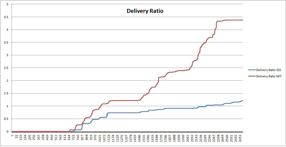
delivery_ratio

This plot simply shows the delivery ratio of the PBR prototcol using the MIT dataset with 103 users, vs the Social Sensing Study data with 26 users. It covers different time periods (both of 1  month), but clips some data at the end of the MIT dataset. However, it does show that the datasets are in some way comparable.

I am continuing to investigate the software, and will speak with Graham (who is in Canada until Christmas) about how best to adapt the software for our needs. It would seem wasteful not to adopt this software which does such a similar thing, without first testing its feasability. Another simulator mentioned by Graham is the ONE simulator, which I have not yet looked at.

What I am also planning to do, is to find out whether the MIT Dataset contains some notion of location, even if that is just cell tower data, that way, it would make it easier to compare any future location based DTN algorithm that we come up with, to Graham’s work, and any other work that uses this dataset.