Matt Stabeler

This graph shows the delivery ratios from the start of the simulation for MIT-OCT dataset. It would appear that in fact, LBR performs poorly against the random algorithm, where the P is the probability of passing on the message (1 copy) to the met node. Interestingly though, when P = 1, the delivery ratio increases. The graphs below show the delivery cost for the different algorithms, spread across two plots, so that the very high costs of Random and Prophet do not dwarf the lower costs of LBR and PBR. These three plots together show that whilst the delivery ratio of  prophet and random are high, the cost is very high.

Delivery costs for three routing algorithms on the MIT-OCT dataset, spread over two plots for clarity.

Perhaps a combined metric for comparison is  cost over delivery ratio, this would perhaps give a better idea of general quality of the algorithm.

I have spent some time looking at the reality mining dataset, to see how useful it is for inferring location about individuals. Firstly I generated a matrix, People over visited cell towers, which was huge, due to the large number of cell towers in the dataset (32, 000). Then I used this data to generate a graph  of people in the dataset, where an edge between two people, if they have ever visited the same cell tower, independantly of whether they were there at the same time. This produced the plot below:

This graph shows people connected based on visiting the same cell towers, but not necessarily at the same time. (full size)

The two plots show the same data, but with well connected node 22 removed on the right. This data implies that most people are using the same cell towers at some points in the dataset, which is promising for using cell tower a  location metric. However, this does not show any information about whether nodes were connected at the same time.

To further clarify the data, I processed the information provided for cell towers, which is stored in two columns in the dataset – oid and name, for example:

I seperated out the cell ids and carrier names  into two columns, which enabled me to get the distribution of carrier names as below:

This shows the number of cells for each known carrier reported in the dataset (30 Others refers to 30 distinct reported carrier names, who’s sum totat was 429 reported towers) (full size)

This suggests that many of the towers are provided by different carriers, so this suggests that, we might have distinct clusters of users, that for some reason are connected by a few – perhaps they ‘roamed’ onto a new network, or changed provider at some point. This needs further clarification, and may only be able to be measured using ‘brute force’, by constructing the graph of people connected based on c0-locations of cell towers.

So far, the analysis is inconclusive, which means it will need a little more investigation. However, my feeling is that we WILL have enough overlap in the dataset to make it feasible to infer location from cell towers records.

Met initially over lunch then in the office. Pádraig had made the following observations:

I think the “Routing with Location” post is very useful for making concrete how location information might help routing. This is the key principle:

“the more locations it visits in common with the destination node, the more likely it will be to pass the message to the destination.”

To be devil’s advocate, the worry would be that the useful information entailed in location is already compiled into the existing contact information. If that is true then the uplift due to the inclusion of location criteria in the routing will not be significant.

Davide and I had been discussing this earlier in the day, and I explained my idea of measuring the importance of a location in terms of how ‘active’ it was; i.e. how many messages exchanges happen there. In this way, it is distinct from contact knowledge alone.

Davide suggested a similar mechanism, which was to measure the popularity of locations, based on, for example the number of different people that visit there. I misssed slightly the meaning when he said an instantaneous value. We talked about concept of maintaining a global table, which tracks the current popularity of locations, and routing to nodes that visit these locations most often.

We discussed the possibility of using the cell tower information contained within the MIT reality mining dataset, and suggested mechanisms for implying location from this. The first, assuming that the nodes are connected to the same network operator, simply being when two nodes are at the same cell tower T1 and T1, they are co-located, else they are not (e.g. they see T1 and T2 respectively)

Another situation to test for however, is when two nodes can ‘see’ each other, but they do not report the same cell tower (T1 ad T2). I suggested a hybrid location, e.g. T12 which is a location where two people have been seen to be connected, but were not connected to the same tower. Initially, we decided to analyse the data to see what it looks like. Pádraig suggested using a simple matrix – People over cell tower IDs with a count of how many times they occur.

One thing we didn’t factor for however, is whether a node can see multiple cell towers at one…. this will become clearer when I have a proper look at the dataset.

Incidentally, this got me thinking about a generic way to represent locations, as 1d, 2d, 3d etc. The MIT dataset cell tower locations, providing all nodes are using the same co-ordindate scheme (i.e. network operator), can be described as a 1d co-ordindate system. The ‘distance’ between points, whilst not meaningful for physical location, could be based on some metric of common movements between locations.

We also talked about ContactSim, and Pádriag agrees that we should probably use this if it is suitable. He asked me to ask Graham for a copy of his chapter that deals with his PBR protocol (Chapter 7) for him to read. We decided that I should try to replicate Graham’s results, to ensure I had a proper handle on what the simulator does.

Pádraid would also like me and Davide(?) to hold a seminar for few people, in which we at least show the results from Grahams work, and discuss the ideas we have about routing with location, I suggested about a year from now, Pádraig was thinking about 2 weeks from now, so in next week’s meeting we will fix the details for the following week.

For next time, I will have replicated Graham’s results, analysed the MIT dataset for applicability for our needs, will have started planning for the seminar, and will have started to adapt Graham’s simulator to use location information.

I have started to look at clustering the location readings into important places. To give me a feel of what the data looks like, I have visualised all of the locations.

Because of the limitations of the browser, it was not possible to visualise all ~40,000 points in the dataset, so it is split into 4 lots of ~10,000. These images are only intended to give a rough idea of how the data is spread out.

My initial thoughts are that there is too much density, and therefore the clustering algorithm has to be highly selective when choosing a place.

Met to discuss the next steps.

Pádraig described a method for testing the quality of a community (i.e. whether it has been partitioned correctly), by means of an infinite(?) random walk, described in a notation based on Huffman(?)  numbers. The length of the decriptions between communities determines the quality of the partitioning. In that a random walk should spend much more time in an actual community, as there are few links out of it. He related this to BUBBLE rap, in that it might be important to test the quality of the communities used in the algorithm, to test how good the community finding algorithm is (e.g. if done on the fly).

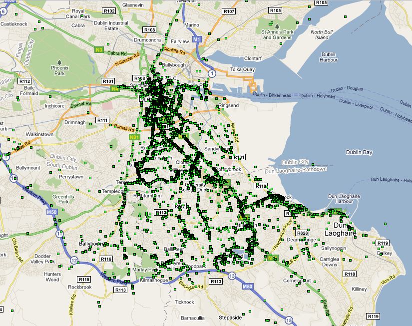
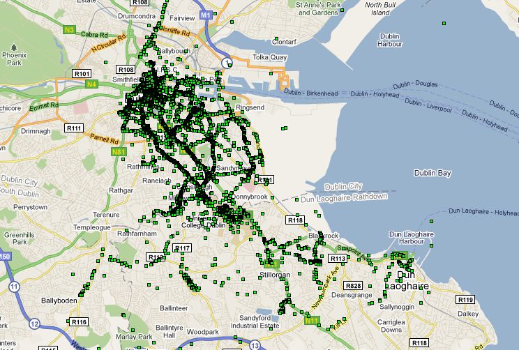
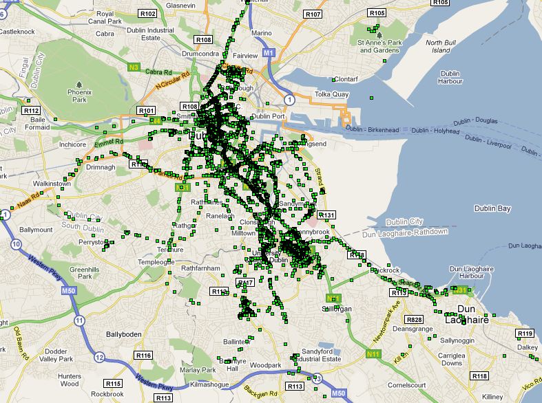
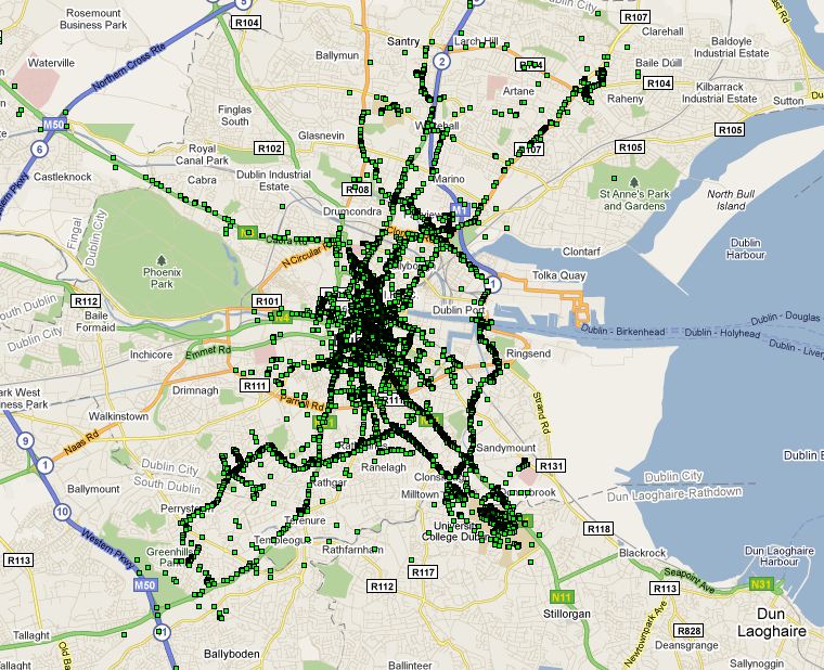
We also spent some time discussing how to define a place, from a series of location readings. Firstly we need to consider whether we determine a location in terms of an individual node, or the global set of readings. After some discussion we decided for the purposes of this simulation, we will determine it globally. This will at least give us an idea about what the data looks like. If it turns out that this seems to produce ‘places’ that encompass too wide an area, we should consider revising this decision.

Sec0ndly, we need to find the means of partitioning the space. We discussed last week clustering the readings using a k-Clique algorithm. I contacted Derek Greene, who supplied me with some links and advice about achieving this. It was his feeling that it was more a distance-based clustering problem, with weighted links, rather than an unweighted k-Clique algorithm (I have yet to explore this), and suggested I initially explore the data using something like MultiDimensional Scaling (MDS), and suggested a Java based implementation.

Davide suggested another approach to the partitioning of locations, in the form of a grid based approach, splitting the landscape based on latitude/longitude, and a size dimension,effectively making a grid of the planet, where all nodes implicitly know that a lat/long is part of a location, if it falls within a grid sqaure.

These two methods have their benefits, the first being that we can get a really good idea about locations based on the data we have, without the worry of partitioning the same place into two locations, in a fairly straightforward way, the second being that all nodes could calculate all possible locations and refer to them when neccassary. We decided in the end to use a clustering algorithm.

I talked through my initial analyis of the Social Sensing Study data, and described how I had found hints of a Bluetooth collection problem, in that for most devices, they had a very low number of instances of device readings. i.e. there were very few occasions when they actually detected Bluetooth devices. This means that using this dataset for detecting proximity using Bluetooth alone may not be very realistic.

(for each type of data, the number of readings out of roughly 89280 possible readings – every 30 seconds for 1 month)

I suggested an alternative solution, using WiFi co-location records instead. (see the paper (cite?!!) that used a similar thing in their evaluation).  I envisage using the logs of WiFi access points in view to determine whether one device is co-located with another. There are three mechanisms for doing this that I thought about afterwards.

1. If two devices can see the same WiFi access point, then they are proximate
2. If two decices can see the same WiFi access points, and the one witht the strongest signal is the same, then they are proximate
3. If the list of WiFi access points that two devices can see overlaps by at least N, then they are proximate

Davide suggested an algorithm that combines these three, which accounts for situations where two nodes are between two wifi points, close to each other, but the signal strength of the WiFi points would result in not being co-located in situation 2 above. Based in the difference between the signal strength of the top 2 (or extended to top N) access points.

We decided that this was worth investigating further.

We talked about an abstract database structure, into which any dataset of this nature could be placed, so that we can compare different datasets. It was much the same as before.

Pádraig suggested that we will need to think about the on-node data structure at some point soon, but that it will be determined by the way that nodes choose to communicate.

Node A:
Visits Loc: L1, l2, l3, l4
Sees Persons: p1, p2, p3
Node B:
Visits Loc: L7, l2, l1, l9
Sees Persons: p2, p8, p6

However, we decided to concentrate first on getting the places clustered, and getting the proxmity records converted into contact windows/periods.

So for the next meeting I said that I would try to have the clustering algorithm implemented and tested on the dataset, as well as checking the bluetooth records issue, and, assuming the data is missing, using the WiFi mechanism to derive contact windows/periods. I also said I would think about the data-structure for the nodes.

Discussed what we should be getting on with:

I will spend some time organising the data from the Social Sensing Study (SSS) and planning an appropriate structure that can be used by any dataset. Around the idea of a table with contact information (e.g. node1 met note 2 at this time) which is assumed to mean that entitied could communicate at that time, and another table which is the place of individual entities over time (e.g. node1 was at location A from T to T’), the place is determined as some labelled k-clustering of raw readings.

There will be some policy decision that will have been made, which determines how data is extracted, these need to be recorded so we can discuss whether they are valid. Can entities communicate only when the raw readings show that they both detected each other, or is  one way detection sufficient. Or how do we detemine the best value of k for clustering.

I will also start to think about how to build a simple simulator that will allow us to test test cases (e.g. send a message at every timestep to every other node to test the limit of the network) for multiple routing algorithms (ideally simultaneously, e.g. BUBBLE and Grahams algorithm).

Also with the idea in mind that datasets, when conforming to this structure, can be tested without having to change code.  By the next meeting I will have come up with some ideas, defined some policies, and will also bring some example data along to inform our choices.

Had a discussion with Davide about what we had decided would be the best algoritm to use as the baseline scenario for routing.

We think the best approach is to use either Graham’s periodic degree routing approach, or the BUBBLE protocol. We sketched out the algorithm for Grahams algorithm, and realised that in fact it is very similar to the BUBBLE protocol, apart from BUBBLE does not adapt to a changing period in which to calculate degree, and Grahams protocol does not use communities.

We also had some ideas about detecting places as higher level concepts of where a node is, rather than raw location readings (e.g. GPS).

We also talked briefly about how we would use the popularity of places, in combination with community knowledge as the basis for a routing algorithm. I will write this up seperately.

Had a first meeting with Padraig, where I presented a few slides (Presentation to Padraig Sep 2010) about my area of interest and how I got to it etc.

Padraig initially suggested that location is not important, but later decided that in fact, it is useful when the network structure is not fully known.

He suggested that I take a baseline scenario, using a reliable dataset (Social Sensing), and use is as a straw man to test further refinements on.E.g. Take the degree approach (Graham & Davide), train it over 1 month, then have a test period, where 50 messages are sent across the network. At the same time have a firm idea about the next stage refinements, i.e. using location to improve routing. (i.e. use a location based routing algorithm). This will then drive the next round of improvements.

He also suggested that the application of the idea is not so important, and whilst I will deal with that in the thesis, it will not figure greatly.

He also talked about community finding in the network, and how we could use that for routing.

I agreed to send on Graham’s paper, and perhaps the BUBBLERap paper.

We will meet again next week.

Had a brainstorm with Davide about what we should analyse. We decide to use the Geolife dataset to test out some ideas:

Firstly I will do a meta-analysis of the data, to see what nodes we do and do not have data for in a given time period. Counting the number of reading per day over the dataset period.

We want to identify the colocation between nodes, and we calculate this

[latex]C_{AB}(t) = 1 - \theta(|x_A(t)-x_B(t)|-\lambda)[/latex]

which means – if A and B are within λ distance of each other (where x is the location of a and y is the location of b) at time t, Cab is 1, else Cab is 0.

[latex]C_{AB} = \frac{1}{T} \sum C_{AB}(t) [/latex]

This gives us the average over all time periods, showing the co-locatedness of a and b. (the sum of the co-location of A and B over all locations, divided by the number of time periods)

We use this to construct a graph, where a and b are connected using a weighted edge labelled with Cab – this network is the structure of co-locatedness, and is exactly the same as a proximity network; it does not care where you meet, only that you do meet.

We calculate this in 1 month(?) blocks to see how the graph evolves over time.

We are also interested to find out if nodes are influential over locations (e.g. if particular nodes visit a location, which then becomes popular).

We plot the popularity of x over time, where the popularity is the number of poeple that visit a location in a day. Where the set of X  is derived from all known locations.We hope to find a pattern where the graph tails off, or increases over time. flat graphs are un-interesting.

For this I will need to calculate locations from the data.

Davide’s note about Mobile Agents

Davide and I have been conducting a quick literature search for interesting papers relating to location in delay tolerant networking, and interesting goals to do with knowledge and prediction of location. The first round led us to four main areas of interest:

• Reccommendation systems
• Routing in Delay Tolerant Networks (obviously)
• Peer-to-peer over proximity networks (e.g. bit torrent over DTN)
• ????

I am in the process of reading a few papers of interest, and Davide is working away at finding other information out. We plan to meet this afternoon to discuss our progress.

I have also parsed and assimilated the GeoLife and Cabspotting datasets, and plan to do the same for the CenceMe dataset.  When we get the Social Sensing project dataset, I will do the same with that. I have tried to use a consistant format for the data, so that when it comes to it, it will be possible to analyse it all in the same way. The simple format is based on the concept that networks are formed of entities, which also have locations that they visit over time.

I had already written, and have since updated to reflect this format, a playback visualisation of entity movements. This is really just a way of seeing what the data looks like over time.

Funding update:

I have finally managed to sort out the details of my funding, and have calculated that I have enough funds to cover a stipend for the next 11 months (I have already paid half fees for this year):

€11,976.42 remaing IRCSET Scholarship fund

+ €2621.25 credit on UCD account – which will be transferred to my IRCSET fund by 18 September 2010

= €14,597.67 / €1333.50 = 10.94 installments.

However, the only problem is that I will not be paid this month, so I plan to ask payroll to produce an advance cheque for this month (fingers crossed).