Matt Stabeler

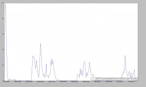
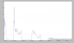
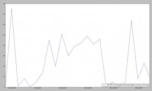
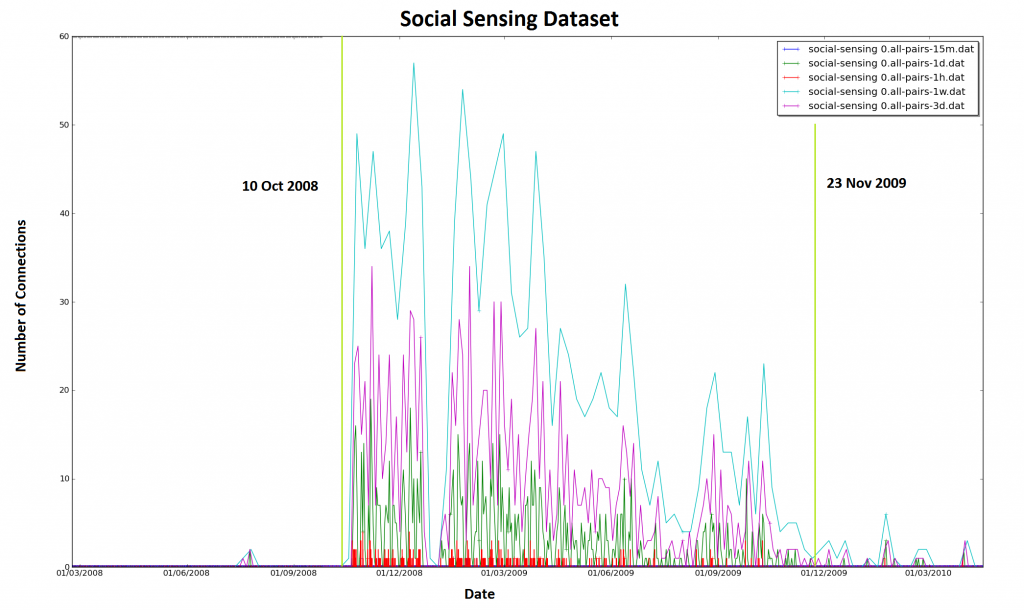
I finally got around to extracting out contact events from the social sensing study. I have made some notes on the Social Sensing Dataset page. The main images are shown below:

Social Sensing Dataset activity, 15mins, hourly, daily, 3 daily, and weekly. Lines showing the most active period

It seems most active from Oct 2008 onwards, and tails off, with the end of Nov 2008 being a good cut-off point. This means there is over a year of contact data.

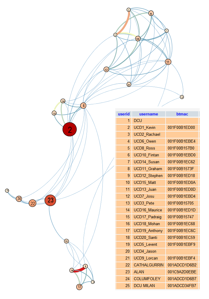
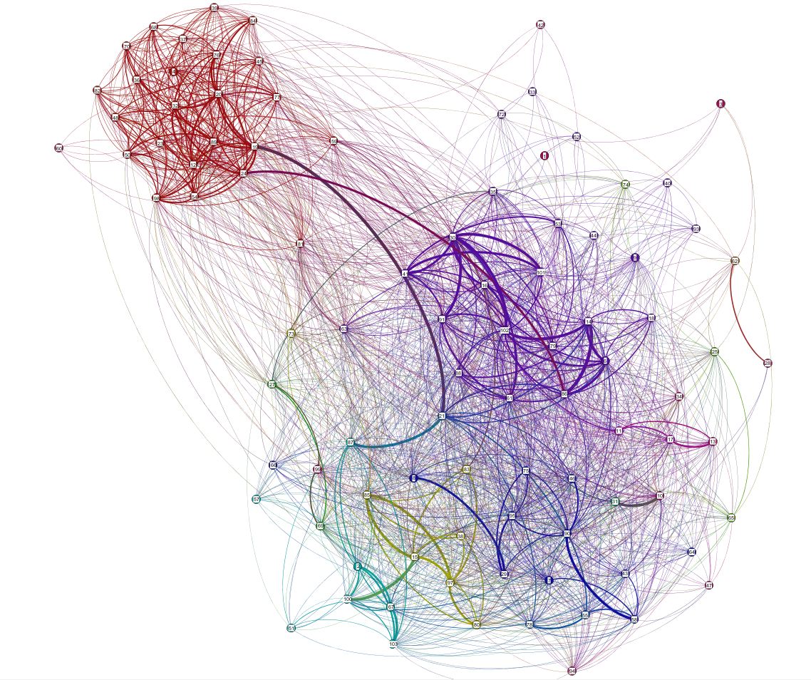
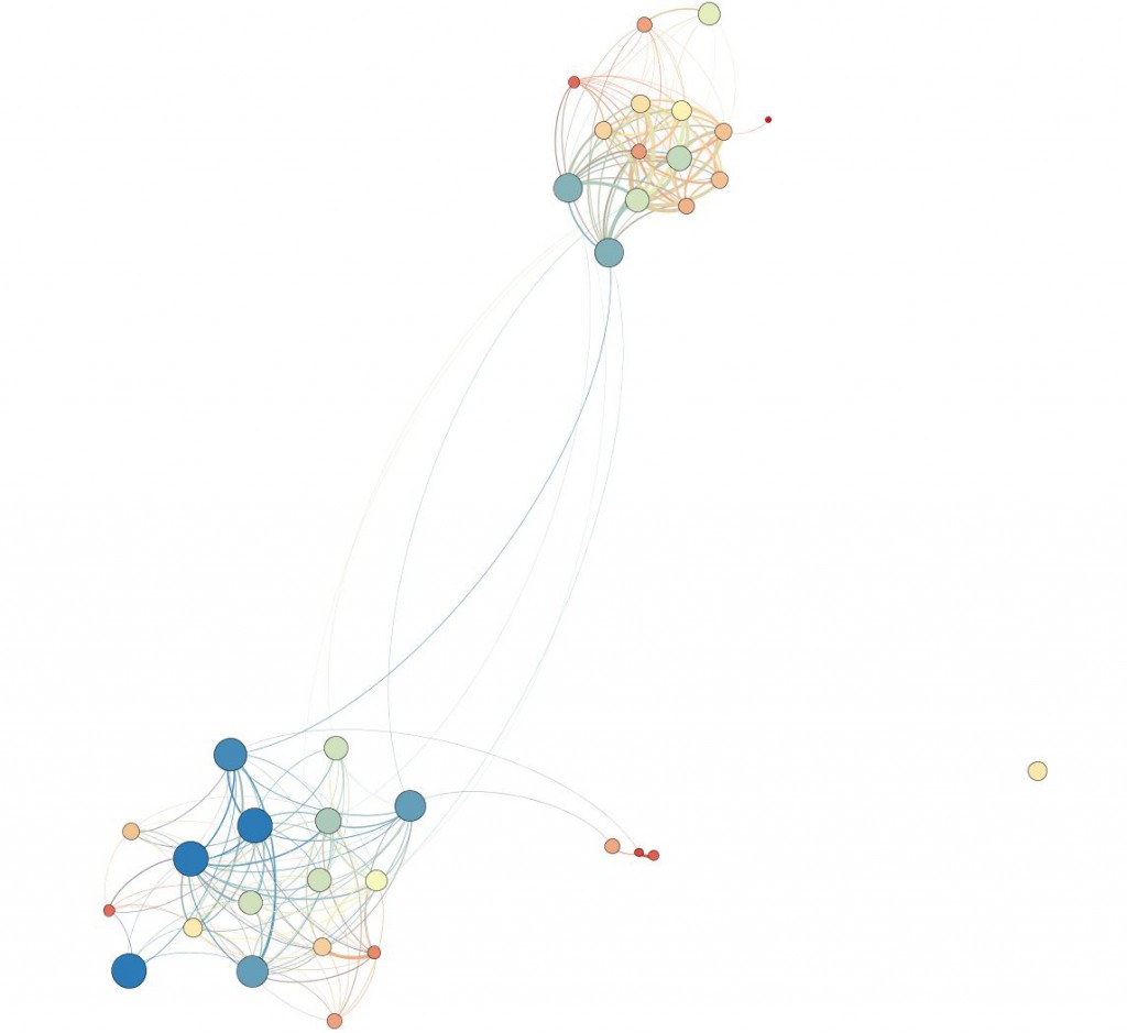
Force directed connected time graph for SocialSensing dataset, showing mapping of users to nodes, with low weight edges removed. NOTE: Do not share this image - remove names/btmacs first

The connected time graph (i.e. edges weighted by the total length of time connected with the target node) gives a really good sense of the social structure. As I personally know most of these people, (and I am on it myself) it is easy for me to see the relevance of the layout.

I haven’t written code to lookup locations based on cell towers/wifi points yet, but it might be interesting in the future if we end up using location.

Also, I need to work on getting BTMAC addresses for the three other people. The problem is that I know that at least one of these people changed phones during the study – hence why they are removed.

There are three (or more) possible routes from this point, either we delve deeper into the merits of using community structure in routing, and try to categorise different networks based on the performance differences of routing in these diverse contact networks. Or we concentrate on the mechanics of making the existing system fully distributed, and therefore having the possibility of real-world deployment. Or we could go down the route of adding a new aspect to the mix, and finding out what location does when put into the mix. However, there is a problem with all of these, and that is that we don’t have the datasets to measure any of them.

Pádraig and I recently discussed relaxing the specification on datasets, to give us larger and more robust data to deal with.

Conrad has a dataset based on wall posts on a social networking site, which we could use as an analogue to a human contact network: A contact event occurs when a wall post is made by one person to another, the ‘duration’ of the contact is based on the length of the wall post.

The Enron dataset has been used in the literature (Kleinberg vector clock paper) before, and we could adapt this in the same way, using the emails to build a network of contacts in a similar way – with message length (if available) as a indicated of contact duration.

Pádraig also mentioned a blogging network, from which we could extract contacts from links, or trackbacks/pingbacks etc.(?)

Finally, the Sentiment project allready collects a large number of tweets, along with location information about them, talking to Anthony Brew, it looks like it may be limited, but I think it is worth a look over the data to see if there is enough coverage to build a reliable network from directed messages (@someone). The problem is that we will only have a percentage of the tweets from the twitter API (apparently). But we could override this by making use of whatever (rate limited) we can get from twitter about an interesting group of specific people, rather than just looking at everyone.

We have decided not to submit to NGMAST11 conference as the results we have were not really ready, also I found an error in the config setup for KCLIQUE BubbleH. I have therefore run all of the simulations from scratch, just to make sure it is all correct. In this re-run, I ran the HGCE algorithms far too many times for each dataset, so there is a very large number of results for the HGCE algorihtm (~700 for each dataset). We plan to submit to the Finding NEMO workshop instead.

To visualise the results so far, we have plotted the best  (see note below) results for BubbleRAP and BubbleH:

BUBBLERap and BubbleH compared for Delivery Ratio, Cost and Latency

To determine the ‘best’ run for algorithms with multiple parameters, we first filtered the results to the best 10 for latency, then ordered by delivery ratio followed by cost, this should mean that a good delivery ratio is still shown for good delivery latency, but avoids results where a abnormally low delivery ratio is chosen with a very poor delivery ratio.

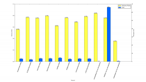
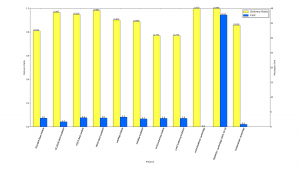
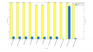
We ran each community finding algorithm over the datasets: MIT-NOV, Cambridge, InfoCom 2005, and InfoCom 2006. We used bubbleRAP, BubbleH, Unlimited flood, hold & wait, and Prophet to measure the effect of the CFA on the dataset. The results below are grouped by dataset. Only the best results for BubbleH/BubbleRAP KCLIQUE and HGCE are shown. Note: The local ranking used for InfoMap is based on the rank given by the InfoMap algorithm, NOT centrality as with BubbleRAP and BubbleH.

MIT-NOV

CAMBRIDGE

IncoCom 2005

InfoCom 2005

My next plan is to link statistics about community structure (number of communities, average members etc.) to the results.

Also, I want to find out if there is an existing measure of overlappiness? Does the amount of overlap in communities affect the results in any way? Also, what about the extent to which there is ‘nesting’ of communities, does this make a difference?

I also want to visualise the communities produced in some way, so that it is clearer what the network structure for the best results is based on.

This excel file this excel file contains the combined results of each CFA for all 4 datasets, so we can compare the effect of community structure (number of communities, average member size) directly with results for each simulation run.

In the last few days, I have been trying out new CFAs for use in the next paper for NGMAST11, the idea behind the paper is exploring different CFAs and datasets and seeing what happens. In order to do this, I have decided to first explore what the Different CFAs do using the MIT-NOV dataset, for both BubbleRAP and BubbleH, i.e. use the communities found by each to drive both DTN algorithm. This gives a fair comparison. Then, I will perform the same tests on different datasets, I envisage problems for some CFAs as the datasets we intend to use are in some cases small, and may not yield good community results, and therefore we will explore thresholding of edges before finding communities (depending on whether the CFA can accept weighted edges or not.

The following tables sum up the tasks invloved, and will be completed as I get the work done:

[TABLE=2]

Some notes so far:

InfoMap undirected, weighted version gives it own ranking for nodes within communities, which can be used in BubbleRAP and BubbleH, so the two versions could be compared. The hierarchical version also does this, but only for the finest level community.

It might be worth writing new community dataset loader for ContactSim/LocationSim so it can take in and calculate the hierarchy, for example, at the moment, each community is defined by a list of nodes, but if we prefix this list with a parent id, it will implicitly specify the hierarchy. (this may be time consuming, but worthwhile down the line, as we can do away with HierarchyOracle and associated classes, and can work directly on communities.

Results so far:

Community finding

InfoMap, which partitions the graph, is easy to visualize,

InfoMap clustering of MIT-NOV dataset - Colour of nodes indicates clustering (edges are coloured by connecting node and weighted by connected time)

The others are harder however, as there I could think of no easy way of indicating all the communities a node belongs to visually, the following shows LinkClustering.

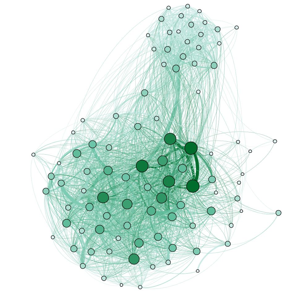
LinkClustering communities on MIT-NOV where the size and colour of the node indicate the number of communities it belongs to

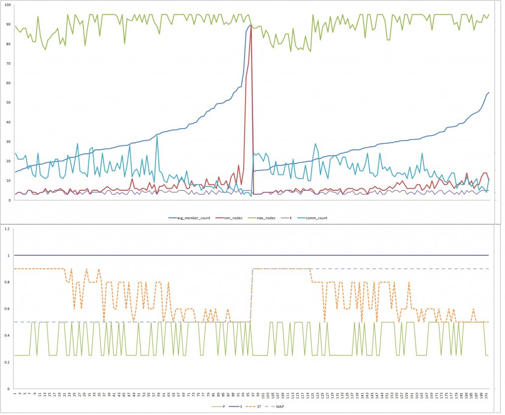
The communities found by HGCE are multiplied across many parameters to the algorithm, so they are much harder to visualise in terms of nodes and edges, however, the plot below, shows the effect on community size and number of communities when changing parameters to HGCE. The graph below is orderded by MAP, ST and average nodes per community. Details about the parameters to HGCE are summarised here.

MIT NOV, HGCE multiple parameters

BubbleH and BubbleRAP

I managed to get a copy of the two InfoCom datasets and the Cambridge dataset  mentioned in the BubbleRAP paper, I could not find the Hong-Kong dataset. I parsed them into the correct format for LocationSim, and was able to genereate edge lists for all the connections, and have vizualised them below. Note: Node size represents betweeness centrality before edge removal. Edge width/colour represents connected time. Graphs below are for mobile nodes only; they do not include fixed nodes.

                 InfoCom05     InfoCom06     Cambridge
#iMotes           41              98             54
     Fixed        0               20             18
     Mobile       41              78             36
External          233             ?              ?
Duration         ~3 days        ~4 days         ~1 month (2 months in readme)

InfoCom 2006 edges removed where connected time less than 4 hours – (min = 1000ms max = 72 hours). InfoCom2006 gephi file.

InfoCom 2006 edges removed where connected time less than 2.5 hours – (min = 1000ms max = 46 hours). infocom2005 gephi file.

Cambridge with edges removed where connected time less than ~3 hours – (min = 1000ms max = ~39 hours). infocom2005 gephi file.

Cambridge Dataset with edges removed where connected time is less than ~3 hours - (min 1000ms max ~39 hours)

These graphs suggest that some community structure exists in the traces, and despite the duration of the InfoCom experiments being quite short, they may have more contact events due to the context of the experiment. (I wonder if the same patterns appear for broad scale deployments that appear in small area deployments?)

TODO:
Plot activity for duration of expermiments.
Parse SocialSensing Dataset…..

Activity every 15 mins for InfoCom2005 datset

Activity every 15 mins for InfoCom2006 datset

Activity every 12 hours for Cambridge dataset

It is important to make sure that each community finding algorithm (CFA) gets a chance to compete on a level playing field, so that they can be equally tested.

The dataset is MIT Reality Mining, which starts in August 200? and ends in May 200?.

The Bubble RAP algorithm uses k-KLIQUE for community finding. The graph contains the core nodes in the dataset, edges are created when a contact is made between two nodes, and labelled with the total time connected between the two nodes. Edges are removed when the total time connected is less than a defined threshold. Then it detects the communities using a k-CLIQUE algorithm, where k = 3. The threshold used by Graham is 2 days. It is 4.5 days in the BubbleRAP paper.

MIT-OCT has been used extensively by Graham, along with MIT-NOV to test his algorithms, so we will continue to use that time period for testing. However, we must make sure that there is sufficient time for all clustering algorithms to make a good effort at finding communities. I believe this was down to the fact that there was activity recorded a large number of users in the dataset for these  time periods.

The figure below shows the average number of connections per week for the whole dataset.

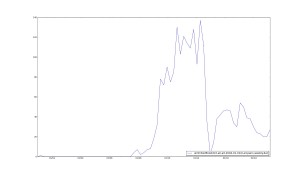
The average number of connections (bluetooth contacts) per week in the MIT Dataset

A note about the MIT-OCT dataset: There are two groups of nodes in the dataset, those belonging to the CORE set, and the rest, which belong to the encompasing ALL set. A node is determined to be in the CORE set if it is part of the MIT Reality Mining study, and is reporting readings. A node that is not in the CORE set, but is in the ALL set, represents a device that has been spotted by a node in the CORE set, but that is not known about apart from it’s contact trace. These are normally considered separate to the routing process, as it would not be possible to communicate with that node.

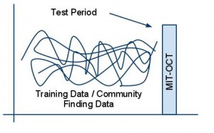
So, for the first experiment, each algorithm will generate communities from 01 Aug 2004 until 27 Sep 2004, and 01 Aug 2004 until 18 Nov 2004. The test period will be  27 Sep 2004 to 25 Oct 2004 and 18 Nov 2004 to 15 Nov 2004.

The image below shows the network generated in the MIT October training period. Some of the low weight (connected time) edges are removed for clarity. It appears to have three groups of nodes.

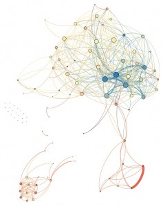
Visualisation of MIT OCT Training edge list. Edges are weighted by the amount of time nodes are connected, with low weight edges removed for clarity. Nodes are sized and coloured by degree.

Some options for community finding algorithms:

• Should the graph they all work on be limited by the threshold period?
  • Justification for this is that BubbleRAP determines this to be important
• Whether or not to use CORE|ALL nodes
• If the CFAs cannot successfully find communities for the training period, we will need to experiment with time periods that suit all algorithms.

The table below shows the results of community finding on the training datsets mit-oct and mit-nov, apart from KCLIQUE which performs very poorly before the end of December for any threshold value, so for the test period,  01 Aug 2004 to 31 Dec 2004 was used to calculate the communities.

* adjusted graph means that some edges were removed from the edge list before passing to the algorithm, in this case, edges where the total connected time of nodes was less than 1 day.

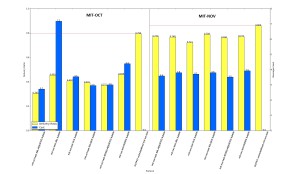
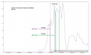
Bubble results for test period Oct and Nov 2004, with training periods 01 Aug 2004 to 27 Sep 2004, and 18 Oct 2004 respectively.

Bubble results for test period Oct and Nov 2004, with training periods 01 Aug 2004 to 27 Sep 2004, and 18 Oct 2004 respectively.

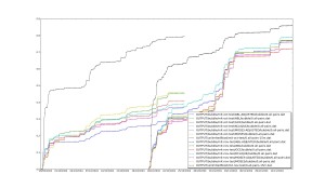
Average weekly connections, showing training period and test period for MIT-OCT and MIT-NOV

Met with Pádraig to talk about next steps, discussed the results so far with the four clustering algorithms. The next steps are:

Tasks

• Stop using the simulation data for community finding.

Posit: all historic data is available and there is a process that is informing community finding, this data is then being used for routing test period.

• Tune GCE so it finds more than 1 community
• (Determine what happens in Bubble-Degree when rank is equal – does it keep or pass) it keeps it – rank must be higher
• Use weighted edges for GCE – Weight based on:
  • Connected time
  • Number of connections
  • Or, threshold as in BubbleRAP
• Use threshold to remove edges for MOSES

If we find that we get improvements based on the community finding algorithm, the next step would be to synthesise some new datasets. Alternative datasets include Cabspotting, Rollernet, Social Sensing.

We could then map out an analysis: message routing that is informed by overlapping community finding, and interesting ways of caculating those communities as time goes by. Towards a paper: ad-hoc message routing based on overlapping communities.

It might also be useful to explore the difference in utility of Overlapping vs Partitioning community finding algorithms.

After a lot of wrangling with code, and spending a good deal of time reading through notes, etc. I was able to work out how to generate community clusters using LocationSim, and how to feed in clusters determined by other mechanisms.

BubbleRAP uses and adapted form of KCLIQUE clustering to generate community structures, along with a score of Betweenness centrality (referred to as Hui Ranking) globally and within clusters to drive the routing process. The adaption relates to the use of a contact threshold, (the Bubblerap paper uses 4.5 days, Graham uses 2 days), which specifies how long on average nodes must be in contact for them to be counted.

I adapted the clustering phase to use MOSES, GCE (using Conrad’s code) and the algorithm by Yong-Yeol Ahn, James P. Bagrow, Sune Lehmann in Link communities in complex networks which I have name ABL. At this stage I have tested only the basic algorithms against MIT-OCT and MIT-ALL node lists.

I found that KCLIQUE does not find any communities for the small time slice in MIT-OCT, this could be because the threshold means that in the course of a month, participants do not spend alot of time together on average.  I will need to explore this further to verify this this.

MOSES and GCE perform badly on the denser, MIT-ALL dataset, and after speaking to Aaron and Conrad, it seems this can be expected with such a closely connected dataset. My next step is to try to use GCE using edge weights, to see if that makes a difference.

in order to get some idea of results for MIT-ALL MOSES and GCE, and MIT-OCT KCLIQUE, I used the communities from their opposite positions to populate the datasets, this meant I was able to simulate BubbleRAP for all cluster types for both MIT-OCT and MIT-ALL.

Another intersting thing I discovered, was Grahams implementation of  Bubble-Degree, which instead of using the Hui Ranking for communities, nodes are ranked by degree over a 6 hour time period. Bubble-Connections worked in the same way but the ranking is based on the number of connections in a 6 hour period. (Graham explains this in section 6.1.2 in his thesis, and in the comments of his code).

The results are below for all cluster types, and both datasets, using bubble-degree, and bubblerap. Also included is unlimited flood to show the maximum possible delivery between all pairs of nodes.

Results for Bubble and Bubble-Degree for dataset MIT-ALL, using KCLIQUE, MOSES, GCE and ABL

Results for Bubble and Bubble-Degree for dataset MIT-OCT, using KCLIQUE, MOSES, GCE and ABL

This seems to suggest that the clustering algoritm does have some effect on the routing algorithm, and further analysis may be able to show whether this is due to simply the difference in number/size of communities.

Other tasks to do:

• Investigate recent improvements of Bubble Rap (if any)
• Consider different network data  (e.g. can we run a similar analysis over a phonecall network?)
• Tweaks to clustering algorithms?
• Chase up SocialSensing dataset
• Continue to think about Location Based Routing – is it feasable still?

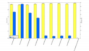
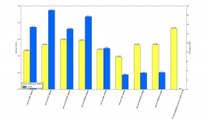
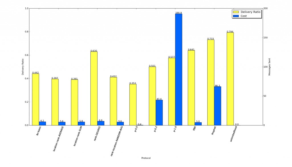
Further to the previous post, I have run some more simulations which include degree rank routing, where individuals are ranked in order based on their degree. I also updated LBR to allow for randomising rank scores, and ran this 25 times to get an idea about the ability for random ranking to deliver messages.

All routing methods shown for comparison.

Interestingly,  routing based on degree only, gives a good delivery ratio. The average of the RANDOM runs performs slightly better than the more sophisticated LBR schemes, but not quite as good as LBR basic (which is the original ranking based solely on cell towers). This suggests to me that the mechanisms we are using to rank locations are not working, perhaps due to lack of rich enough data. It will be interesting to see how this dataset compares to other datasets.